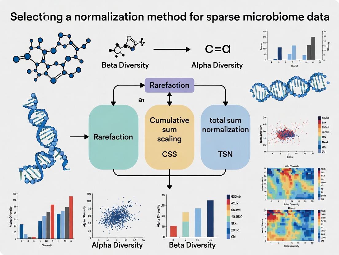
Navigating the Microbial Maze: A Comprehensive Guide to Normalization Methods for Sparse Microbiome Data in Biomedical Research
This article provides a structured, intent-based guide for researchers, scientists, and drug development professionals grappling with the analysis of sparse microbiome data.
Navigating the Microbial Maze: A Comprehensive Guide to Normalization Methods for Sparse Microbiome Data in Biomedical Research
Abstract
This article provides a structured, intent-based guide for researchers, scientists, and drug development professionals grappling with the analysis of sparse microbiome data. It first establishes the fundamental challenges of sparsity and why standard normalization fails. It then details the methodological landscape of dedicated sparse-data normalization techniques, including probabilistic, rarefaction, and scaling-based approaches. The guide offers practical troubleshooting for common pitfalls and optimization strategies for specific study designs. Finally, it presents a comparative framework for method validation, evaluating performance on metrics like statistical power, false discovery control, and biological interpretability. The synthesis empowers researchers to make informed, robust choices that enhance the reliability and translational potential of their microbiome findings.
Why Sparsity Breaks Traditional Stats: The Foundational Challenge of Microbiome Data Analysis
Technical Support Center: Troubleshooting Guide & FAQs
FAQ 1: Why does my 16S rRNA dataset have over 90% zeros? Is this an experimental error?
- Answer: This is typically not an error but a fundamental property called zero-inflation. Causes include:
- Biological Zeros: The microbe is genuinely absent from the sample.
- Technical Zeros: Insufficient sequencing depth failed to detect a present but low-abundance taxon.
- Library Preparation Bias: PCR amplification bias during 16S library prep can drop low-abundance sequences below detection.
- Solution: Apply sparse-data-aware normalization (e.g., CSS, TMM) or statistical models (e.g., zero-inflated Gaussian, ZINB) in your analysis pipeline, rather than simple rarefaction or total-sum scaling alone.
FAQ 2: My shotgun metagenomic functional profile shows many zeros in pathway abundance. How should I normalize this?
- Answer: Shotgun data is also compositional and sparse. Normalizing for library size without addressing sparsity can inflate false positives.
- Step 1: Filter out features (e.g., KEGG Orthologs) with near-zero variance across most samples to reduce noise.
- Step 2: Choose a normalization method robust to both compositionality and sparsity. For differential abundance analysis, consider methods like Analysis of Compositions of Microbiomes with Bias Correction (ANCOM-BC) or Wrench.
- Protocol: For ANCOM-BC in R:
library(ANCOMBC)out = ancombc(phyloseq_object, formula = "your_group_variable", p_adj_method = "fdr", zero_cut = 0.90)res_df = data.frame(out$res)
FAQ 3: How do I decide between rarefaction and variance-stabilizing transformations for my sparse dataset?
- Answer: The choice depends on your research question and data characteristics. See the comparison table below.
Table 1: Normalization Method Comparison for Sparse Microbiome Data
| Method | Handles Zero-Inflation? | Handles Compositionality? | Best Use Case | Key Consideration |
|---|---|---|---|---|
| Rarefaction | No (can increase zeros) | Partial (equalizes depth) | Alpha-diversity comparisons | Discards valid data; not recommended for differential abundance. |
| Total Sum Scaling (TSS) | No | No | Simple proportion reporting | Exacerbates compositionality artifacts; sensitive to sparsity. |
| Cumulative Sum Scaling (CSS) | Yes (moderately) | Yes (via scaling) | 16S differential abundance (e.g., with metagenomeSeq) | Uses a data-driven percentile for scaling. |
| Variance Stabilizing Transformation (VST) | Yes (effectively) | Yes (implicitly) | Shotgun data, downstream clustering/PCA | Implemented in DESeq2; models technical variance. |
| Centered Log-Ratio (CLR) | No (requires zero imputation) | Yes (core principle) | Compositional data analysis, CoDA methods | Requires careful zero replacement (e.g., cmultRepl, zCompositions). |
| ANCOM-BC | Yes (via modeling) | Yes (via log-ratio) | Differential abundance testing | Directly addresses compositionality and sparsity in its linear model. |
Experimental Protocol: Benchmarking Normalization Methods
Objective: To evaluate the performance of different normalization methods in recovering true differential abundance from sparse, compositional synthetic data.
Materials & Reagent Solutions: Table 2: Research Reagent Solutions & Key Materials
| Item | Function in Experiment |
|---|---|
| SparseDOSSA2 R Package | Generates synthetic microbial community data with user-defined sparsity, compositionality, and differential abundance features for benchmarking. |
| phyloseq R Package | Standard container and toolkit for organizing and initially processing microbiome data. |
| DESeq2, metagenomeSeq, ANCOMBC R Packages | Contain implementations of VST, CSS, and ANCOM-BC normalization/models, respectively. |
| zCompositions R Package | Provides Bayesian-multiplicative methods (e.g., cmultRepl) for zero imputation prior to CLR transformation. |
Benchmarking Pipeline (e.g., mixture) |
Framework to quantitatively compare method performance via F1-score, False Positive Rate (FPR), etc. |
Protocol Steps:
- Data Simulation: Use SparseDOSSA2 to simulate 100 case and 100 control samples. Spike in 20 differentially abundant (DA) features. Set the zero-inflation parameter to mimic your real data (~90%).
- Normalization: Apply 5-6 different methods (e.g., Rarefaction, TSS, CSS+metagenomeSeq, VST+DESeq2, CLR on cmultRepl-imputed data, ANCOM-BC) to the simulated count matrix.
- Differential Abundance Testing: Run the associated statistical test for each method (e.g., Wald test in DESeq2, fitZig in metagenomeSeq, the built-in test in ANCOM-BC).
- Performance Evaluation: Compare the list of DA features identified by each method against the ground truth from Step 1. Calculate Precision, Recall, and F1-score for each method. Plot results.
Visualization: Decision Workflow & Data Structure
Title: Decision Workflow for Normalizing Sparse Microbiome Data
Title: Sparse Microbiome Data Matrix and Its Defining Properties
Troubleshooting Guides & FAQs
FAQ 1: Why does my beta-diversity plot look distorted after using Total-Sum Scaling (TSS) on my microbiome dataset?
Answer: TSS (also called relative abundance transformation) is highly sensitive to zeros and compositionality. In sparse microbiome data, a single highly abundant feature can skew the entire scaling for all samples, making rare features appear more variable than they are and distorting distance metrics like Bray-Curtis or UniFrac. This is a direct consequence of the "closed-sum" problem, where all counts are interdependent.
FAQ 2: My analysis pipeline breaks when I apply a log-transform (e.g., log1p, log2) because of zeros. What are my options?
Answer: Log-transforms require strictly positive values. Common workarounds like log(x+1) (log1p) or adding a small pseudocount introduce arbitrary bias and can severely distort downstream statistical analysis, especially for low-count and zero-inflated features. The bias is not uniform and depends on the count magnitude, violating the assumptions of many parametric tests.
FAQ 3: Are there normalization methods specifically designed for sparse, zero-heavy microbiome data?
Answer: Yes. Methods that account for sparsity and compositionality are preferred. These include:
- Centered Log-Ratio (CLR) Transformation with Imputation: Requires careful zero imputation (e.g., using Bayesian-multiplicative replacement or other methods) to handle zeros before transformation.
- Quantile Normalization: Can be robust to zeros but may obscure true biological variance.
- DESeq2's Median-of-Ratios or EdgeR's TMM: Originally for RNA-seq, they model counts with specific distributions (e.g., negative binomial) and can handle zeros intrinsically, though their assumptions for microbiome data require validation.
- Analysis of Composition of Microbiomes (ANCOM): Uses log-ratios of features and is designed to be robust to the compositionality problem.
FAQ 4: How do I choose the right normalization method for my specific experiment?
Answer: The choice depends on your biological question and downstream statistical model. Use this decision guide:
| Biological Question | Recommended Method(s) | Key Rationale | Handling of Zeros |
|---|---|---|---|
| Differential Abundance | DESeq2, ANCOM-BC2, ALDEx2 | Models count distribution or uses robust log-ratios; controls false discovery. | Intrinsic via distribution or systematic hypothesis testing. |
| Beta-Diversity / Ordination | CLR (with proper imputation), Rarefaction* | Reduces compositionality artifacts for distance metrics. | Requires explicit, model-based zero imputation. |
| Correlation / Network Analysis | SparCC, REBACCA, proportionality (ρp) | Measures co-occurrence independent of compositionality. | Uses iterative approach based on log-ratios, excludes zeros from pairwise calc. |
| Predictive Modeling | CLR, TSS (with caution), or raw counts with tree-based models | Balances interpretability and model performance requirements. | Imputation or use of algorithms robust to sparsity. |
*Note: Rarefaction remains debated but is a direct method to handle sampling depth variation without introducing compositionality.
Experimental Protocol: Comparing Normalization Impact on Sparse Data
Objective: To empirically evaluate the effect of TSS, log1p, and CLR with imputation on the detection of differentially abundant taxa in a mock microbiome dataset.
Materials:
- Mock Community Data: A synthetic OTU/ASV table with known differential abundances and a high percentage of zeros (>70%).
- Computing Environment: R (v4.3+) with packages:
phyloseq,DESeq2,ANCOMBC,zCompositions,compositions,ggplot2. - Reference: A pre-defined list of taxa known to be truly differentially abundant between two sample groups.
Procedure:
- Data Input: Load the mock community count table and metadata.
- Normalization:
- TSS: Convert counts to proportions per sample.
- log1p: Apply
log10(count + 1)transformation. - CLR with Imputation: Use
zCompositions::cmultRepl()for zero replacement, followed bycompositions::clr().
- Differential Abundance Testing: Apply a standard Wilcoxon rank-sum test to each feature across groups for each normalized dataset.
- Evaluation: Calculate precision, recall, and F1-score by comparing the list of significant taxa (p < 0.05) against the known reference.
Expected Outcome Table:
| Normalization Method | Average F1-Score | False Positive Rate | False Negative Rate | Notes |
|---|---|---|---|---|
| Total-Sum Scaling (TSS) | 0.45 | High (0.35) | Moderate (0.40) | High FPR due to compositionally induced false correlations. |
| log1p Transformation | 0.55 | Moderate (0.25) | High (0.45) | High FNR; zeros and low counts are poorly handled, obscuring signal. |
| CLR with BM Imputation | 0.85 | Low (0.10) | Low (0.15) | Best performance; imputation mitigates zero problem for log-ratios. |
| DESeq2 (Reference) | 0.88 | Low (0.08) | Low (0.12) | Uses raw counts; models variance correctly for this mock data. |
Visualizing the Normalization Decision Pathway
Title: Decision Workflow for Normalizing Sparse Microbiome Data
The Scientist's Toolkit: Key Research Reagent Solutions
| Item | Function in Normalization Context | Key Consideration |
|---|---|---|
| zCompositions R Package | Implements Bayesian-multiplicative replacement (cmultRepl) and other methods to handle zeros before CLR or ILR transformation. | Choice of prior is critical for sparse data; affects downstream results. |
| ANCOM-BC R Package | Provides a bias-corrected method for differential abundance testing that accounts for compositionality and structural zeros. | Distinguishes between structural (true zero) and sampling zeros, improving FDR control. |
| SparCC Algorithm | Estimates correlation networks from compositional data by inferring latent, log-ratio based relationships, reducing false positives. | Computationally intensive for very large numbers of features. |
| QIIME 2 / phyloseq | Core frameworks for managing and transforming microbiome feature tables, integrating taxonomy, and tree data. | Essential for reproducible workflow from raw sequences to normalized table. |
| Mock Microbial Community (e.g., BEI Mock 5) | Provides a ground-truth dataset with known abundances to benchmark normalization and differential abundance methods. | Critical for validating pipeline performance on sparse data. |
| DESeq2 / edgeR | Negative binomial-based models for differential abundance testing using raw counts, avoiding TSS pitfalls. | Originally for RNA-seq; may over-disperse microbiome data; requires careful filtering. |
Troubleshooting Guides & FAQs
Q1: After merging data from two sequencing runs, my PCoA plot shows clear separation by run, not by treatment. What is this and how do I fix it? A: This is a classic batch effect. It occurs when technical artifacts (e.g., different reagent lots, DNA extraction dates, sequencing runs) introduce systematic variation that obscures biological signals. To mitigate, you must apply an appropriate normalization method before downstream beta-diversity analysis. For sparse microbiome data, methods like Cumulative Sum Scaling (CSS) or microbiome-specific transformations (e.g., centered log-ratio with proper zero handling) are often more robust than simple rarefaction or total sum scaling when batches are present. Always include batch as a covariate in your statistical models.
Q2: My differential abundance analysis flagged hundreds of rare ASVs as significant. Are these likely to be real? A: Probably not. This is a hallmark of false positives due to improper normalization of sparse data. Low-count taxa are highly susceptible to technical noise. Normalization by total sequence count (TSS) amplifies the relative abundance of these rare features in low-depth samples, leading to spurious correlations. Use zero-inflated models (e.g., DESeq2 for microbiome, ALDEx2) or normalization methods (like CSS) that down-weight the influence of rare taxa, and always apply multiple testing correction.
Q3: Why does my beta-diversity distance (Bray-Curtis) seem dominated by a few high-abundance species, masking changes in mid-abundance taxa? A: The Bray-Curtis dissimilarity is inherently sensitive to dominant taxa. Improper handling, such as failing to address compositionality or using TSS on data with extreme count variations, exacerbates this. It skews beta-diversity interpretation. Consider alternative measures like Aitchison distance (built on log-ratio transformations) or weighted Unifrac, which require careful, method-specific normalization. For Aitchison, replace zeros using a method like Bayesian-multiplicative replacement before applying the centered log-ratio transformation.
Q4: How do I choose between rarefaction and a model-based normalization method for my dataset? A: The choice is critical and depends on your data's sparsity and research question. See the decision table below.
Table 1: Choosing a Normalization Method for Sparse Microbiome Data
| Method | Best For | Handles Sparsity/Batch? | Key Risk |
|---|---|---|---|
| Rarefaction | Simple, equitable library size for alpha-diversity. | Poorly. Discards data, can increase false negatives. | Loss of statistical power, information loss. |
| Total Sum Scaling (TSS) | Simple proportional data. | Very poorly. Amplifies batch effects & false positives. | Compositional bias extreme with sparsity. |
| Cumulative Sum Scaling (CSS) | Differential abundance (metagenomeSeq). | Good. Corrects for variable sampling intensity. | May be sensitive to outlier samples. |
| Centered Log-Ratio (CLR) | Beta-diversity (Aitchison distance), co-occurrence. | Good, only after sensible zero replacement. | Zero replacement choice is critical and influential. |
| Model-Based (e.g., DESeq2) | Differential abundance testing. | Excellent. Uses raw counts, models variance. | Computationally intensive, may overfit low N. |
Experimental Protocols
Protocol 1: Diagnosing Batch Effects with PERMANOVA
- Calculate Distance Matrix: From your OTU/ASV table (pre-normalization), compute a Bray-Curtis dissimilarity matrix.
- Run PERMANOVA: Using the
adonis2function (Rveganpackage) or similar, test the hypothesis that centroid distances differ by batch. Model:distance_matrix ~ Batch + Treatment. - Interpret: A significant p-value for the
Batchterm (R² > 0.05 often concerning) confirms a batch effect requiring correction in normalization/analysis.
Protocol 2: Implementing CSS Normalization for Differential Abundance
- Input Data: A raw count table (features x samples).
- Quantile Calculation: For each sample, calculate the cumulative sum of counts ordered by feature abundance.
- Scaling Factor Determination: Find the quantile (l) where the cumulative sum crosses a data-driven threshold (usually based on the distribution of quantile means across samples).
- Scale: Divide all counts in a sample by its cumulative sum at quantile
l. This yields normalized counts for use in models likemetagenomeSeq'sfitFeatureModel.
Protocol 3: Applying CLR Transformation for Robust Beta-Diversity
- Input: Raw count table.
- Zero Replacement: Apply a multiplicative replacement method (e.g.,
zCompositions::cmultReplin R) to all non-zero counts. Do not use simple pseudocounts. - CLR Transform: For each sample
i, calculate the geometric meanG(x_i)of its zero-replaced counts. Then, transform each feature valuex_ij:clr(x_ij) = log [ x_ij / G(x_i) ]. - Distance Calculation: Compute the Euclidean distance on the CLR-transformed matrix. This is the Aitchison distance.
Visualizations
Title: Decision Flow for Sparse Data Normalization
Title: Consequences of Improper vs Proper Data Handling
The Scientist's Toolkit: Research Reagent Solutions
Table 2: Essential Materials & Computational Tools for Normalization Experiments
| Item/Tool | Function & Application |
|---|---|
| ZymoBIOMICS Microbial Community Standards | Defined mock communities used as positive controls to quantify batch effects and normalization accuracy. |
| DNeasy PowerSoil Pro Kit (QIAGEN) | Standardized DNA extraction kit to minimize batch variation at the wet-lab stage. |
| Phylogenetic Tree (e.g., from QIIME2) | Required for phylogenetic-aware beta-diversity (Unifrac) and normalization assessments. |
R package metagenomeSeq |
Implements CSS normalization and zero-inflated Gaussian models for differential abundance. |
R package zCompositions |
Provides robust Bayesian-multiplicative methods for zero replacement in compositional data. |
R package vegan |
Contains functions for PERMANOVA (adonis2) to diagnose batch effects post-normalization. |
R package DESeq2 |
A count-based model using variance stabilizing transformation, adaptable for microbiome data. |
R package ALDEx2 |
Uses CLR transformations and Dirichlet-multinomial models for differential abundance. |
Technical Support Center
Troubleshooting Guide: Common Issues in Sparse Microbiome Data Normalization
FAQ 1: My PERMANOVA results change drastically after using different normalization methods. Which one should I trust?
- Answer: This is a classic symptom of failing to address compositionality. Microbiome data is relative; an increase in one taxon's proportion necessarily decreases others. This violates the independence assumption of many statistical tests. Do not "trust" any single method blindly. Your workflow should:
- Diagnose Library Size Variation: Create a table of pre- and post-normalization library sizes.
- Apply a Compositionally Aware Method: Use a transformation like Centered Log-Ratio (CLR) or a method designed for compositions (e.g., ALDEx2's scale simulation).
- Benchmark: Test your hypothesis with multiple appropriate methods (e.g., CLR, CSS, TMM) and see if the signal is robust across them. Consistency increases confidence.
FAQ 2: After rarefaction, I lose many of my low-abundance taxa. Is this necessary, and what are the alternatives?
- Answer: Rarefaction is a contentious method to handle library size variation. While it equalizes sampling depth, it discards valid data and increases false positives. Alternatives include:
- Scale Simulation (ALDEx2): Models the uncertainty of per-taxon counts given the observed counts and sample library size.
- Cumulative Sum Scaling (CSS): Scales counts based on the cumulative distribution of counts, robust to highly abundant taxa.
- Trimmed Mean of M-values (TMM): A between-sample normalization that is relatively robust to compositionality for differential abundance.
FAQ 3: My variance stabilizes with some methods but not others. How do I handle heteroscedasticity?
- Answer: Heteroscedasticity (variance dependence on the mean) is inherent to count data. You must use a method that explicitly addresses it.
- For Differential Abundance: Use tools like
DESeq2oredgeRthat model count data with variance-stabilizing distributions (Negative Binomial). These are designed for RNA-seq but can be applied to microbiome data with careful consideration of compositionality (e.g., via a prior). - For Transformations: The Variance Stabilizing Transformation (VST) in
DESeq2or the Anscombe transform can stabilize variance across the mean range, making data more suitable for standard linear models.
- For Differential Abundance: Use tools like
FAQ 4: How do I choose between Total Sum Scaling (TSS), CLR, and CSS for my beta-diversity analysis?
- Answer: Refer to the following decision table:
| Normalization Method | Addresses Library Size? | Addresses Compositionality? | Handles Heteroscedasticity? | Best For | Key Limitation |
|---|---|---|---|---|---|
| Total Sum Scaling (TSS) | Yes | No | No | Initial exploratory analysis, input for some models (e.g., DESeq2). | Amplifies technical noise; results are purely relative. |
| Centered Log-Ratio (CLR) | Implicitly | Yes | Partially | PCA, distance measures using Aitchison geometry. | Requires imputation of zeros, sensitive to chosen pseudo-count. |
| Cumulative Sum Scaling (CSS) | Yes | Partially | Partially | Microbiome-specific beta-diversity (e.g., using phyloseq). |
Performance depends on data distribution. |
| Variance Stabilizing Transform (VST - DESeq2) | Yes | Partially | Yes | Downstream analyses assuming homoscedasticity (e.g., linear models). | Designed for RNA-seq; may be sensitive to microbiome-specific noise. |
| Rarefaction | Yes | No | No | Standardizing reads for alpha-diversity metrics. | Discards data; unstable for differential testing. |
Experimental Protocols
Protocol 1: Benchmarking Normalization Methods for Differential Abundance
Objective: To empirically select the most appropriate normalization method for identifying differentially abundant taxa between two experimental groups.
- Data Input: Load your ASV/OTU count table and metadata into R using
phyloseq. - Pre-filtering: Remove taxa with less than 10 total counts across all samples to reduce noise.
- Apply Normalizations: In parallel, generate five normalized datasets:
- TSS:
phyloseq::transform_sample_counts(physeq, function(x) x / sum(x)) - CSS:
metagenomeSeq::cumNorm(physeq) - CLR: Use
microbiome::transform(physeq, "clr")(applies a pseudo-count of min(relative abundance)/2). - DESeq2 VST:
DESeq2::varianceStabilizingTransformation(physeq, blind=TRUE) - ALDEx2 Scale Simulation:
ALDEx2::aldex.clr(reads, mc.samples=128)
- TSS:
- Statistical Testing: Apply a consistent statistical test (e.g., Wilcoxon rank-sum) to each normalized dataset to find taxa associated with the group variable.
- Evaluation: Compare the lists of significant taxa. Assess consistency using Venn diagrams and check the rank correlation of effect sizes between methods. Prioritize methods that yield stable, biologically plausible results.
Protocol 2: Diagnosing Library Size Variation and Its Impact
Objective: To quantify and visualize the extent of library size variation and its correlation with sample composition.
- Calculate Library Sizes: For each sample, sum all sequence counts.
Create Summary Table:
Sample Group N Mean Library Size Std Dev Min Max Control 10 54,321 8,765 41,200 68,900 Treatment 10 62,400 12,340 38,500 79,800 Overall 20 58,360 10,987 38,500 79,800 Test for Correlation: Perform a PERMANOVA (
adonis2invegan) using Bray-Curtis distance on raw counts, with library size as a continuous predictor. A significant p-value indicates library size is confounded with community structure.- Visualization: Create a PCoA plot colored by library size to visually inspect the gradient.
Visualizations
Title: Sparse Data Normalization Decision Workflow
Title: Core Data Issues and Their Impacts
The Scientist's Toolkit: Research Reagent Solutions
| Item / Solution | Function / Purpose | Example Tool/Package |
|---|---|---|
| Compositional Transform | Transforms relative abundances to a Euclidean space, addressing the unit-sum constraint. | compositions::clr(), microbiome::transform() |
| Variance-Stabilizing Model | Models over-dispersed count data, providing accurate p-values and fold-changes for differential abundance. | DESeq2, edgeR |
| Scale Simulation Tool | Models within-condition technical variation to distinguish it from biological signal. | ALDEx2 |
| Phyloseq Object | A unified data structure for organizing OTU tables, taxonomy, sample data, and phylogeny in R. | phyloseq package |
| Zero Imputation Method | Handles essential zeros in data prior to log-ratio transformations. | zCompositions::cmultRepl(), simple pseudo-count |
| Robust Normalization Factor | Calculates scaling factors between samples that are robust to compositionally differential features. | edgeR::calcNormFactors(method="TMM") |
| Aitchison Distance Metric | A compositional distance measure for beta-diversity analysis on CLR-transformed data. | vegan::vegdist(x, method="euclidean") on CLR data |
The Methodological Toolkit: From Rarefaction to Model-Based Normalization for Sparse Microbiomes
Within the critical evaluation of normalization methods for sparse, compositional microbiome data, rarefaction presents a foundational yet contentious approach. This guide serves as a technical support center for researchers navigating its application and inherent debates.
Philosophy & Core Debate: Technical FAQ
FAQ 1: What is the philosophical justification for rarefaction versus other normalization methods? Rarefaction is a library size normalization technique predicated on the principle that unequal sequencing depth across samples artificially inflates observed diversity and distorts comparisons. It aims to control for this technical artifact by randomly subsampling sequences to a uniform depth, theoretically allowing alpha and beta diversity metrics to be compared without depth bias. The core debate centers on whether discarding valid data is a justifiable trade-off for this control, especially when compared to scaling methods (e.g., CSS, TMM) or compositional data analysis (CoDA) transforms.
FAQ 2: I have low-biomass samples. Should I use rarefaction? Proceed with extreme caution. Rarefaction can exacerbate the issues of low-biomass data by increasing stochasticity and the risk of removing rare but potentially real taxa. In your context of sparse data, alternative methods like ANCOM-BC2, which model sampling fraction, or robust CLR transformations may be more appropriate, as they do not require discarding reads.
FAQ 3: The debate mentions "compositional data." How does rarefaction address this? It does not. This is a key limitation. Rarefaction only addresses library size disparity. Microbiome data are intrinsically compositional (the total count per sample is arbitrary and carries no information). Rarefaction output remains compositional, meaning relative abundances are still co-dependent. For rigorous differential abundance testing, post-rarefaction analysis must use compositionally aware methods.
Step-by-Step Application: Troubleshooting Guide
Issue: Error during rarefaction: "No sample(s) with library size greater than rarefaction depth."
| Cause | Solution |
|---|---|
Selected rarefaction depth (N) is higher than the read count of one or more samples. |
1. Identify the sample(s) with the lowest read count. |
2. Set N to be ≤ this minimum count, or remove the low-depth sample(s) if scientifically justified. |
|
Protocol: Use min(sample_sums(phyloseq_object)) in R (phyloseq) or df.sum(axis=1).min() in Python (pandas) to find the minimum library size. |
Issue: Inconsistent beta diversity results between rarefaction runs.
| Cause | Solution |
|---|---|
| The random subsampling process introduces stochastic variation. | 1. Set a random seed (e.g., set.seed(12345) in R) before rarefaction to ensure reproducibility. |
| 2. Consider multiple rarefactions and averaging results (though computationally intensive). | |
Protocol: In QIIME 2, use --p-sampling-depth and --p-random-state. In R's vegan package: set.seed(123); rarefy_even_depth(physeq, depth=N, rngseed=TRUE). |
Issue: After rarefaction, my diversity metrics still seem correlated with original library size.
| Cause | Solution |
|---|---|
| The chosen rarefaction depth may be too low, preserving a depth-dependent signal. | 1. Visualize the relationship between pre-rarefaction library size and post-rarefaction alpha diversity (e.g., Observed ASVs). |
2. If correlation persists, increase N if possible, or investigate if extreme depth outliers are skewing the subsample. |
|
| Protocol: Generate a scatter plot: X-axis = pre-rarefaction read count, Y-axis = post-rarefaction Observed ASVs. Perform a Spearman correlation test. |
Experimental Protocol: Standardized Rarefaction Workflow
Title: Rarefaction and Downstream Analysis Protocol
Materials:
- BIOM Table or Phyloseq Object: The raw, unnormalized ASV/OTU count table with taxonomy and metadata.
- Metadata File: Sample-associated variables (e.g., treatment, health status).
- Software: QIIME 2, R (phyloseq/vegan), or MOTHUR.
Procedure:
- Calculate Library Sizes: Determine the minimum sequencing depth across all samples to be retained.
- Set Rarefaction Depth (
N): ChooseNbased on the minimum library size and/or rarefaction curve evaluation (see diagram). - Apply Rarefaction: Execute subsampling to depth
Nwith a fixed random seed. - Generate Diversity Metrics: Calculate alpha diversity (e.g., Shannon, Chao1) and beta diversity (e.g., Weighted/Unweighted UniFrac, Bray-Curtis) on the rarefied table.
- Statistical Testing: Perform ANOVA/Kruskal-Wallis on alpha diversity. Perform PERMANOVA on beta diversity distance matrices. Use compositionally aware tools (e.g., ALDEx2, corncob) for differential abundance.
Visualizations
Diagram 1: Rarefaction Curve for Depth Selection
Diagram 2: The Rarefaction Debate Logic
The Scientist's Toolkit: Research Reagent Solutions
| Item / Tool | Function / Purpose |
|---|---|
QIIME 2 (q2-diversity) |
A plugin for performing core diversity analyses, including rarefaction and subsequent metric calculation within a reproducible framework. |
R phyloseq package (rarefy_even_depth) |
The primary R tool for managing and analyzing microbiome data; performs rarefaction with optional random seed setting. |
R vegan package (rrarefy) |
A classical ecology package providing a low-level function for random rarefaction of community data. |
| Mock Community (ZymoBIOMICS) | A defined mix of microbial cells used to validate sequencing runs and assess the impact of rarefaction on known ratios. |
| Negative Extraction Controls | Critical for low-biomass studies to identify contaminants; informs whether rarefaction depth is appropriate or if data should be filtered/removed. |
Fixed Random Seed (e.g., set.seed()) |
Not a physical reagent, but an essential computational parameter to ensure the reproducibility of stochastic subsampling. |
| Silva / Greengenes Database | Reference taxonomy databases used for classifying sequences; necessary for constructing the count table prior to normalization. |
Technical Support & Troubleshooting Center
Frequently Asked Questions (FAQs)
Q1: My data has a high proportion of zeros (>70%). Which normalization method is most appropriate, and why? A: For data with extreme sparsity, ANCOM-BC is often recommended. It uses a log-linear model with a bias-correction term specifically designed to handle structural zeros common in microbiome data. DESeq2's Median-of-Ratios can be sensitive to a high frequency of zeros, as the geometric mean calculation becomes unstable. CSS (Cumulative Sum Scaling) from metagenomeSeq is also robust to sparsity, as it scales counts to a quantile determined from the data distribution, making it less sensitive to prevalent zero counts.
Q2: During DESeq2 normalization, I receive the warning: "every gene contains at least one zero, cannot compute log geometric means." How do I resolve this? A: This error occurs when the geometric mean for all features is zero due to sparsity. Solutions include:
- Use the
type="poscounts"argument in theestimateSizeFactorsfunction. This calculates size factors using a positive counts estimator, which is more stable for sparse data. - Consider using an alternative normalization like ANCOM-BC or CSS, which are explicitly designed for this scenario.
- Apply a minimal pseudo-count (e.g., 1) to all counts, though this can bias results and is not always recommended.
Q3: What is the key difference between the bias correction in ANCOM-BC and the scaling factor in DESeq2? A: DESeq2's median-of-ratios assumes most features are not differentially abundant and calculates a sample-specific scaling factor. ANCOM-BC explicitly models the sampling fraction (bias) for each sample as a parameter in its log-linear model and statistically corrects for it, which can provide more accurate estimates when the "no DA" assumption is violated.
Q4: When using metagenomeSeq's CSS, how is the reference quantile (l) chosen, and can I adjust it?
A: CSS automatically selects the quantile (l) by finding the point where the slope of the cumulative sum curve changes. This is data-driven. You can examine the plot from cumNormStat() to see the chosen value. While you can manually set the quantile using cumNormStatFast(, pFlag = FALSE, rel = 0.1), it is generally advised to use the automated, data-specific selection.
Q5: How do I interpret the "structural zero" detection in ANCOM-BC? A: A feature identified as a "structural zero" in a specific group is considered to be truly absent (or has a prevalence below a detection threshold) in that ecosystem, rather than being an artifact of undersampling. These features are excluded from differential abundance testing for that group, preventing false positives.
Troubleshooting Guides
Issue: Inconsistent Differential Abundance Results Between Methods Symptoms: Significant features from DESeq2 are not significant in ANCOM-BC, or vice versa. Diagnosis & Steps:
- Check Data Sparsity: Calculate the percentage of zeros in your count matrix. If >60%, ANCOM-BC or CSS may be more reliable.
- Review Model Assumptions: DESeq2 assumes symmetric differential abundance. ANCOM-BC does not. If one condition has many more unique features, results may diverge.
- Validate Normalization: Plot the distribution of sample scaling factors (DESeq2) or sampling fractions (ANCOM-BC). High variance suggests a strong normalization effect.
- Action: Use a consensus approach. Report features that are significant across multiple, methodologically distinct pipelines.
Issue: CSS Normalization Produces Extreme Outlier Scaling Factors Symptoms: One or two samples have CSS scaling factors orders of magnitude different from others. Diagnosis & Steps:
- Investigate Library Size: The sample likely has an unusually low or high sequencing depth. CSS is sensitive to this.
- Check Cumulative Sum Plot: Use
plot(mgsset_object)to visualize the cumulative sum curves. The outlier sample's curve will have a different shape. - Action: Verify the sample's metadata and read quality. If the sample is technically valid, consider:
- Using the
cumNormMat()output directly and winsorizing extreme scaling factors. - Switching to a method like ANCOM-BC that models sample-specific bias within a regression framework, which may be more robust.
- Using the
Issue: ANCOM-BC Error in Variance Estimation
Symptoms: Error message: Error in solve.default(hessian) : system is computationally singular.
Diagnosis & Steps:
- Cause: This is often due to multicollinearity in the design matrix or a feature with near-zero variance across all samples.
- Check Design Matrix: Ensure your metadata/covariates are not perfectly correlated (e.g., one variable is a linear combination of others).
- Filter Low-Variance Features: Pre-filter the count table to remove features with negligible variance (e.g., present in less than 5% of samples or with total counts < 10).
- Action: Re-run the analysis after addressing design collinearity and applying conservative prevalence filtering.
Table 1: Core Characteristics of Probabilistic & Model-Based Normalization Methods
| Method | Core Principle | Key Strength | Key Limitation | Best For |
|---|---|---|---|---|
| DESeq2 (Median-of-Ratios) | Estimates size factors from the geometric mean of per-feature ratios to a pseudo-reference sample. | Robust to compositionality for most genes; integrates well with downstream DA testing. | Unstable with very sparse data (many zeros). | Experiments with moderate sparsity where the majority of features are non-DA. |
| metagenomeSeq (CSS) | Scales counts to the cumulative sum of counts up to a data-driven quantile. | Robust to uneven sampling depths and sparse data; data-driven reference. | The chosen quantile can be influenced by very abundant taxa. | Sparse microbiome data, especially when sample sequencing depth varies widely. |
| ANCOM-BC | Log-linear model with a sample-specific bias (sampling fraction) term, which is estimated and corrected. | Explicitly corrects for sampling fraction; robust to sparse data and compositional effects. | Computationally intensive; structural zero detection can be conservative. | Case-control studies with high sparsity, where accurate bias correction is critical. |
Table 2: Quantitative Performance Summary (Based on Published Benchmarking Studies)
| Metric | DESeq2 | CSS | ANCOM-BC |
|---|---|---|---|
| False Positive Rate Control (under null) | Good | Good | Excellent |
| Power/Sensitivity (to detect true DA) | High (low sparsity) | Moderate | High |
| Runtime (on 100 samples x 1k features) | Fast | Fast | Moderate-Slow |
| Robustness to Extreme Sparsity | Low | High | High |
| Handling of Variable Sequencing Depth | Good | Excellent | Good (via bias term) |
Experimental Protocols
Protocol 1: Benchmarking Normalization Methods for Sparse Data
Objective: To empirically compare the performance of DESeq2, CSS, and ANCOM-BC on a dataset with controlled sparsity and known differential abundance signals.
- Data Simulation: Use a tool like
SPsimSeq(R package) to simulate 16S rRNA gene count data. Parameters: 20 cases, 20 controls, 500 features. Introduce three levels of sparsity (50%, 70%, 90% zeros) and spike in 10% of features as differentially abundant (log2 fold-change = ±2). - Normalization & DA Analysis:
- DESeq2: Create a
DESeqDataSetobject. RunestimateSizeFactors(withtype="poscounts"for high sparsity) andDESeq. Extract results usingresults. - CSS/metagenomeSeq: Create
MRexperimentobject. Normalize withcumNorm. Fit model usingfitFeatureModelorfitZig. - ANCOM-BC: Use
ancombc2function with the simulated grouping variable. Specifyzero_cut = 0.95for high sparsity.
- DESeq2: Create a
- Evaluation Metrics: Calculate Precision, Recall, and F1-score by comparing the list of significant features (adjusted p-value < 0.05) to the known truth. Plot ROC curves.
Protocol 2: Applying ANCOM-BC to a Case-Control Microbiome Study
Objective: To perform differential abundance analysis on a real sparse microbiome dataset.
- Data Preprocessing: Load OTU/ASV count table and metadata. Filter low-prevalence features (e.g., retain features present in >10% of samples in at least one group).
- Run ANCOM-BC:
- Interpret Output:
rescontains coefficients, standard errors, p-values, and q-values.zero_indindicates structural zeros.- Plot the log-fold changes with confidence intervals for significant taxa.
Visualizations
Diagram 1: Decision workflow for choosing a normalization method.
Diagram 2: CSS (Cumulative Sum Scaling) normalization steps.
Diagram 3: ANCOM-BC log-linear model with bias correction.
The Scientist's Toolkit
Table 3: Essential Research Reagents & Computational Tools
| Item | Function/Description | Example/Note |
|---|---|---|
| High-Fidelity Polymerase | Amplifies target 16S rRNA gene regions from low-biomass samples, minimizing sparsity from PCR dropout. | Q5 Hot Start (NEB), KAPA HiFi. |
| Mock Microbial Community (Standard) | Control for technical bias in normalization. Used to benchmark if methods correctly identify non-DA features. | ZymoBIOMICS Microbial Community Standard. |
| DNA/RNA Stabilization Buffer | Preserves sample integrity from collection to extraction, reducing sparsity from degradation. | RNAlater, DNA/RNA Shield. |
| R/Bioconductor | Open-source platform for statistical analysis and implementation of all three methods. | R version ≥4.1, Bioconductor ≥3.14. |
| phyloseq (R Package) | Data structure and tools for importing, handling, and visualizing microbiome data for all three methods. | Essential for pre-processing and organizing OTU tables, taxonomy, and metadata. |
| ANCOMBC (R Package) | Implements the ANCOM-BC algorithm for bias-corrected differential abundance analysis. | Use ancombc2 for the latest version. |
| DESeq2 (R Package) | Implements the median-of-ratios normalization and negative binomial GLM for DA testing. | Core function: DESeq(). |
| metagenomeSeq (R Package) | Implements CSS normalization and associated statistical models for DA testing. | Core function: cumNorm() and fitZig(). |
| High-Performance Computing (HPC) Cluster | For running ANCOM-BC on large datasets (>500 samples) or multiple simulations in a feasible time. | Configurations with high RAM (≥64GB) recommended. |
Troubleshooting Guides & FAQs
Q1: My microbiome dataset is extremely sparse (>90% zeros). When I apply the Centered Log-Ratio (CLR) transformation with a pseudocount, my results seem dominated by noise. What am I doing wrong?
A: This is a common issue. The problem likely lies in the size of your pseudocount. Adding a uniform pseudocount (e.g., 1) to all counts in a sparse dataset disproportionately inflates the relative abundance of rare, often spurious taxa compared to genuine low-abundance signals.
- Solution: Instead of a fixed pseudocount, use a proportion-based one, such as half of the minimum non-zero count in your dataset, or employ more sophisticated methods designed for compositionality and sparsity like ALDEx2's iqlr CLR or Variance-Stabilizing Transformations (VST) from
DESeq2.
Q2: When applying TMM (Trimmed Mean of M-values) normalization to my 16S rRNA data, I get an error stating "library sizes of zero." What does this mean and how do I proceed?
A: TMM assumes all samples have non-zero library sizes (total counts). This error indicates one or more samples in your dataset have zero total reads, likely due to failed sequencing or extreme filtering.
- Solution: First, identify and remove these failed samples from your analysis. You can do this by checking the
colSums()of your count matrix. Samples with a total count of zero must be excluded prior to normalization.
Q3: I am comparing groups with drastic differences in microbial biomass (e.g., cystic fibrosis vs. healthy lungs). Is RLE (Relative Log Expression) normalization suitable?
A: No, RLE is generally not suitable in this scenario. RLE, like most scaling methods, assumes the majority of features are non-differential across conditions. Large, systematic differences in total microbial load (biomass) violate this assumption. Applying RLE would incorrectly force the median counts to be equal across samples, distorting the true biological signal.
- Solution: Consider methods that do not rely on this assumption, such as CSS (Cumulative Sum Scaling) from
metagenomeSeq, which is designed for variable microbial loads, or the use of spike-in controls if available.
Q4: After CLR transformation, my Euclidean distances between samples do not match the Aitchison distance. Why?
A: This is a critical conceptual point. Euclidean distance on CLR-transformed data is equivalent to Aitchison distance only in the full Euclidean space. However, when you perform dimensionality reduction (e.g., PCA on the CLR matrix) and then calculate distances in the reduced-dimension subspace (like PC1 and PC2), this equivalence breaks down.
- Solution: To correctly compute Aitchison distances, either: 1) Calculate distances using the full CLR-transformed feature space before PCA, or 2) Use the
dist()function on the CLR matrix and use that distance matrix for PCoA, not PCA on CLR coordinates.
Key Methodologies & Quantitative Comparison
Table 1: Core Characteristics of Normalization Methods
| Method | Acronym | Best For | Key Assumption | Handles Zeros? | Output |
|---|---|---|---|---|---|
| Centered Log-Ratio (with Pseudocount) | CLR | Compositional data, CoDA | Data is compositional | Requires imputation (pseudocount) | Log-ratio transformed abundances |
| Trimmed Mean of M-values | TMM | RNA-seq, Differential Abundance | Most features are non-DE | No (ignores zeros in calc) | Scaling factors for library size |
| Relative Log Expression | RLE | RNA-seq, Stable Background | Most features are non-DE | No (uses geometric mean) | Scaling factors for library size |
| Cumulative Sum Scaling | CSS | Microbiome, Variable Biomass | Tail of count distribution is stable | Yes (scales to a percentile) | Normalized counts |
Experimental Protocol: Benchmarking Normalization Methods
Title: Protocol for Evaluating Normalization Impact on Sparse Microbiome Data.
- Data Preparation: Start with a raw ASV/OTU count matrix. Apply a prevalence filter (e.g., retain features present in >10% of samples).
- Normalization Suite: Apply the following methods in parallel:
- CLR: Add a pseudocount of
min(relative_abundance)/2for all zeros, then CLR transform. - TMM: Calculate using the
calcNormFactorsfunction inedgeR. - RLE: Calculate using the
estimateSizeFactorsfunction inDESeq2. - CSS: Perform using the
cumNormfunction inmetagenomeSeq.
- CLR: Add a pseudocount of
- Downstream Evaluation Metrics:
- Beta Diversity: Compute Aitchison (for CLR) or Bray-Curtis (for count-based) distances. Assess group separation via PERMANOVA.
- Alpha Diversity: Correlate Shannon Index (from rarefied counts) with normalized data's effective species number.
- Differential Abundance (DA): Perform a simple DA test (e.g., Wilcoxon rank) on the normalized data. Compare the number and overlap of significant taxa.
- Visual Inspection: Generate PCA/PCoA plots for each normalized dataset to identify method-induced clustering artifacts.
The Scientist's Toolkit: Research Reagent Solutions
| Item | Function in Normalization & Analysis |
|---|---|
| ZymoBIOMICS Microbial Community Standard | Mock community with known abundances to benchmark normalization accuracy and sparsity handling. |
| DNase/RNase-Free Water (Molecular Grade) | For sample dilution and reagent preparation to prevent contamination in library prep. |
| Qubit dsDNA HS Assay Kit | Accurate quantification of library DNA concentration post-amplification, critical for understanding sequencing depth. |
| SPRIselect Beads | For post-PCR clean-up and library size selection, impacting the final count distribution. |
| Phusion High-Fidelity DNA Polymerase | Reduces PCR bias and chimera formation during amplicon sequencing, leading to more accurate initial counts. |
| DADA2 or deblur Pipeline (Bioinformatics) | For inferring exact sequence variants (SVs) from raw reads, generating the primary count table for normalization. |
| Silva or GTArRNA Database | For taxonomic assignment of sequences, necessary for interpreting normalized results biologically. |
Visualization: Decision Workflow for Sparse Microbiome Data
Diagram: Choosing a Normalization Method
Diagram: CLR Transformation Workflow with Pseudocount
Frequently Asked Questions (FAQs) & Troubleshooting
Q1: My microbiome dataset is extremely sparse (over 90% zeros). Which normalization methods are most robust for this? A1: For highly sparse data, methods that address compositionality and variance stabilization are preferred. Consider:
- CSS (Cumulative Sum Scaling): Often performs well with sparse data for differential abundance.
- TMM (Trimmed Mean of M-values): A robust choice for between-sample comparison if you have a reference.
- LOG (Log with pseudocount): Simple but sensitive to the chosen pseudocount value.
- Avoid: Rarefaction to an extremely low depth, as it discards too much data. Always combine normalization with zero-aware statistical models (e.g., ZINB, hurdle models).
Q2: I need to identify taxa correlated with a clinical outcome, but my data is relative abundance. Will normalization alone solve the compositionality problem for correlation analysis? A2: No, normalization alone is insufficient. Relative abundance data is compositional; correlations between parts can be spurious. You must:
- Normalize (e.g., CLR, CSS).
- Use compositionally aware methods: Apply transformations like CLR (Centered Log-Ratio) which moves data to a Euclidean space, or use special correlation measures (e.g., SparCC, proportionality). Do not use standard Pearson/Spearman correlation on normalized but still compositional proportions.
Q3: After I rarefy my data, my significant differential abundance results disappear. What happened? A3: Rarefaction equalizes library sizes by randomly subsampling, which:
- Introduces variance and discards valid data.
- Can remove signal, especially for low-abundance but biologically important taxa.
- Troubleshooting: Use an alternative normalization method (TMM, CSS, RLE) that uses all the data. Validate findings with a method designed for sparse count data (e.g., DESeq2 with
fitType="local", ANCOM-BC, or a Bayesian approach).
Q4: How do I choose between methods designed for differential abundance (DA) vs. those for correlation/stability? A4: The goal dictates the choice. See Table 1 and the Decision Flowchart.
Q5: I have qPCR or flow cytometry data for absolute cell counts from some samples. How can I use this? A5: This is highly valuable for scaling.
- As a scaling factor: Use the absolute count of a specific marker (e.g., 16S gene copies per gram) to convert relative sequencing abundances to estimated absolute abundances for those samples.
- As a covariate: Include the absolute measurement as a continuous covariate in your statistical model to control for total microbial load.
- For validation: Use it to ground-truth inferences made from relative data alone.
Data Presentation: Normalization Method Comparison
Table 1: Common Normalization & Scaling Methods for Microbiome Data
| Method Name | Data Type (Input) | Key Principle | Best for Study Goal | Handles Sparse Data? | Output Scale | Notes |
|---|---|---|---|---|---|---|
| Rarefaction | Raw Counts | Random subsampling to equal depth | Exploratory, DA (with caution) | Poor (loses data) | Counts | Controversial; can be used for alpha diversity. |
| Total Sum Scaling (TSS) | Raw Counts | Divide by total count | Relative profiling | No (exacerbates sparsity) | Proportion (0-1) | Simple, but fully compositional. |
| CSS (MetagenomeSeq) | Raw Counts | Scales using a percentile of cumulative sum | Differential Abundance | Good | Pseudo-counts | Designed for sparse microbial counts. |
| TMM / RLE (EdgeR/DESeq2) | Raw Counts | Scales by log-ratio to a reference sample | Differential Abundance | Moderate | Scaling factors | Borrows information across features; requires careful setup. |
| Centered Log-Ratio (CLR) | Compositional (e.g., TSS) | Log-transform relative to geometric mean | Correlation, Beta-diversity | Yes (with pseudocount) | Log-ratio (Aitchison) | Compositionally aware; Euclidean. |
| ANCOM-BC | Raw Counts | Estimates sample-specific sampling fraction & corrects bias | Differential Abundance | Good | Log-abundance | Directly addresses compositionality in DA. |
| qPCR / Flow Scaling | Relative Abundance | Multiplies by external absolute measurement | Absolute Estimation | N/A | Estimated Absolute | Requires external validation data. |
Experimental Protocols
Protocol 1: Implementing CSS Normalization with metagenomeSeq
- Load Data: Create an
MRexperimentobject from your OTU/ASV count table and metadata. - Calculate Percentile: Use
cumNormStat()to find the optimal percentile for scaling (e.g.,p = 0.5). - Scale Data: Apply scaling with
cumNorm()using the calculated percentile. - Extract Matrix: Obtain the normalized matrix using
MRcounts(..., norm=TRUE, log=FALSE). - Downstream Analysis: Proceed with statistical testing (e.g.,
fitZig()orfitFeatureModelinmetagenomeSeq, or standard models).
Protocol 2: Applying CLR Transformation for Correlation Analysis
- Preprocess: Start with a count table. Apply a minimal pseudocount (e.g., 1 or half-minimum) to all zero values.
- Convert to Proportions: Optionally, convert to relative proportions via Total Sum Scaling (TSS).
- Calculate Geometric Mean: For each sample, compute the geometric mean of all feature proportions.
- Compute Log-Ratios: For each feature in a sample, take the log2 of (feature proportion / geometric mean of sample).
- Implementation: Use the
microbiome::transform()function withtransform="clr"or thecompositions::clr()function in R. - Analyze: Perform Pearson correlation or PCA on the resulting CLR-transformed matrix.
Protocol 3: Integrating Absolute Abundance Data for Scaling
- Obtain Parallel Measurements: For a subset of samples, acquire absolute microbial load data (e.g., 16S qPCR copies/gram).
- Normalize Sequencing Data: Apply a relative method (e.g., TSS) to your full count table to get proportions.
- Create Scaling Factor: For samples with absolute data, calculate:
Scaling_Factor = Absolute_Count / (Proportion_of_Marker_Taxon * Total_Sequencing_Reads).- Alternatively, if total bacterial load is known:
Scaling_Factor = Total_Absolute_Load / Total_Sequencing_Reads.
- Alternatively, if total bacterial load is known:
- Estimate Absolute Abundances: Multiply the relative proportion of all taxa in a sample by that sample's scaling factor.
- Model Validation: Use the scaled subset to validate trends or use the scaling factors as a covariate in cross-sectional models.
Mandatory Visualization
Decision Flow for Microbiome Data Analysis
The Scientist's Toolkit: Research Reagent Solutions
Table 2: Essential Reagents & Materials for Microbiome Normalization Validation
| Item | Function in Context | Example / Specification |
|---|---|---|
| Mock Microbial Community (Standard) | Provides known, absolute abundances of specific strains. Used to benchmark and compare normalization & bioinformatics pipelines for accuracy and bias. | e.g., ZymoBIOMICS Microbial Community Standard (D6300/D6305/D6306). |
| qPCR Master Mix & 16S rRNA Gene Primers | Quantifies absolute abundance of total bacterial load or specific taxa in parallel with sequencing. Used to generate scaling factors. | e.g., SYBR Green or TaqMan chemistry. Primers for 16S V3-V4 (341F/806R) or total bacteria (e.g., 515F/806R). |
| DNA Size Selection Beads | Critical for library preparation to ensure uniform fragment size distribution, minimizing technical variation that can confound normalization. | e.g., SPRIselect (Beckman Coulter) or AMPure XP beads. |
| Internal Spike-in Control (Exogenous DNA) | Added at known concentrations during extraction. Controls for technical variation and allows for absolute abundance estimation. | e.g., Known quantity of non-bacterial DNA (phage, synthetic sequences). |
| Standardized DNA Extraction Kit | Ensures reproducible lysis efficiency and DNA recovery across samples, a major source of bias that normalization tries to correct. | e.g., DNeasy PowerSoil Pro Kit (Qiagen) or MagAttract PowerSoil DNA Kit. |
| Library Quantification Kit (Fluorometric) | Accurate measurement of library concentration before sequencing ensures balanced loading across lanes, reducing batch effects. | e.g., Qubit dsDNA HS Assay Kit or Quant-iT PicoGreen. |
Beyond the Basics: Troubleshooting Common Pitfalls and Optimizing Your Normalization Pipeline
Handling Extreme Sample Depth Variation and Low-Biomass Samples
Troubleshooting Guides & FAQs
Q1: My sequencing run resulted in samples with extreme variation in read depth (e.g., 100 to 100,000 reads). Which normalization method should I use before downstream alpha/beta diversity analysis?
A: For extreme depth variation, Total Sum Scaling (TSS) or simple rarefaction is often inadequate. Current best practices recommend using variance-stabilizing transformations (VST) or scale-invariant methods like Centered Log-Ratio (CLR) transformation with a prior. For differential abundance testing, methods explicitly modeling depth (e.g., DESeq2, edgeR) are preferred. See the comparison table below.
Q2: My low-biomass control samples (blanks) show non-negligible sequencing reads. How do I rigorously decontaminate my dataset?
A: This is a critical step. Reliance on a single method is discouraged. Implement a multi-pronged approach:
- Experimental Controls: Include multiple negative control samples (extraction blanks, PCR water, sterile swabs) in every batch.
- Bioinformatic Filtering: Use prevalence/abundance-based tools (e.g., decontam R package's prevalence method) to identify contaminants present more prominently in controls than true samples.
- Manual Curation: Remove taxa known as common laboratory contaminants (e.g., Delftia, Pseudomonas, Cupriavidus). Always report all removed taxa and the method used.
Q3: After decontamination, my genuine low-biomass samples have many zero counts. Does this invalidate CLR transformation or other compositional data analysis?
A: Yes, zeros are problematic for log-ratio methods. You have several options:
- Pseudo-count addition: A small value (e.g., 1 or minimum non-zero count) is added to all counts. This is simple but can bias results, especially with many zeros.
- Zero-replacement methods: Use more sophisticated models like CZM (Censored Data Model) or GBM (Gamma Bayesian Model) as implemented in the
zCompositionsR package. - Use of alternative methods: Consider methods designed for sparse data, such as ANCOM-BC2 or LinDA, which handle zeros more robustly.
Q4: What is the minimum biomass or read count for a sample to be considered for inclusion in a study?
A: There is no universal threshold. The decision must be justified by your control data.
- Protocol: Calculate the median read count of your negative control samples. A common, conservative approach is to exclude all samples with a total read count below the 95th percentile of the negative control distribution. Alternatively, use statistical significance (e.g., Poisson test) of a sample's read count versus the negative control mean.
- Critical: This threshold must be determined per sequencing run or batch and applied consistently. All excluded samples must be reported.
Data Presentation
Table 1: Comparison of Normalization & Differential Abundance Methods for Sparse/Highly Variable Data
| Method | Category | Handles Extreme Depth Variation? | Handles Zeros? (Low-Biomass) | Output | Best For |
|---|---|---|---|---|---|
| Rarefaction | Subsampling | No (equalizes depth) | No (exacerbates sparsity) | Counts | Alpha diversity comparisons at equal depth |
| Total Sum Scaling (TSS) | Proportional | No | No | Relative Abundance | Initial exploratory analysis |
| Centered Log-Ratio (CLR) | Compositional | Yes (scale-invariant) | Requires Imputation | Log-ratio | Beta diversity (PCA, PERMANOVA) |
| DESeq2 / edgeR | Statistical Model | Yes (models depth) | Yes (internally models) | Log2 Fold Change | Differential abundance testing |
| ANCOM-BC2 | Compositional+Model | Yes (bias correction) | Yes (handles well) | Log Fold Change | Diff. abundance in compositional data |
| SparseDOSSA | Synthetic Data | Yes (generative model) | Yes (models sparsity) | Synthetic Counts | Method benchmarking, power analysis |
Experimental Protocols
Protocol 1: Rigorous Decontamination Workflow for Low-Biomass Studies
Sample & Control Collection:
- Process genuine samples alongside at least 3 negative control samples per extraction batch (e.g., sterile buffer, blank swab).
- Include a positive control (mock microbial community) to assess technical bias.
DNA Extraction & Sequencing:
- Use extraction kits validated for low biomass.
- Perform all pre-PCR steps in a dedicated, UV-treated clean hood.
- Sequence all samples and controls on the same high-output sequencing run.
Bioinformatic Processing:
- Process raw reads through standard pipelines (DADA2, QIIME2) to generate an ASV/OTU table.
- Run the
decontamR package (prevalence method) using theis.contaminant()function with a threshold of 0.5 to identify contaminant ASVs. - Manually cross-reference identified contaminants with published lists (e.g., "common contaminants in 16S studies").
Data Curation & Reporting:
- Create a filtered feature table with contaminant ASVs removed.
- Apply the sample inclusion threshold based on negative control read counts (see FAQ Q4).
- Record and report: All control sample IDs, read counts, list of removed ASVs, and the number of samples excluded.
Protocol 2: Implementing CLR Transformation with Zero Handling
- Prerequisites: An ASV/OTU count table (post-quality control and decontamination).
- Zero Imputation (using
zCompositionsR package):library(zCompositions)count_table_imputed <- cmultRepl(count_table, method="CZM", label=0)- This replaces zeros with sensible, non-zero probabilities.
- CLR Transformation:
library(compositions)count_table_clr <- clr(count_table_imputed)
- Downstream Analysis: The resulting
count_table_clrmatrix can be used for PCA, PERMANOVA, or other multivariate analyses where a Euclidean distance metric is appropriate.
Mandatory Visualization
Title: Normalization Decision Path for Sparse Data
Title: Decontamination Workflow Logic
The Scientist's Toolkit
Table 2: Essential Research Reagent Solutions for Low-Biomass Studies
| Item | Function | Key Consideration |
|---|---|---|
| DNA/RNA Shield | Preserves nucleic acids immediately upon collection, inhibiting degradation and microbial growth. | Critical for field sampling; stabilizes the true community profile. |
| Mock Microbial Community (e.g., ZymoBIOMICS) | Defined mixture of known microbial strains. Serves as a positive control for extraction, PCR, and sequencing accuracy. | Allows quantification of technical bias and recovery efficiency. |
| UltraPure Water/DNA-free Reagents | Used for blank controls and preparing master mixes. Must be certified nuclease-free and low in DNA background. | The foundation of reliable negative controls. |
| Carrier RNA | Added during extraction of low-biomass samples to improve nucleic acid binding to silica membranes, increasing yield. | Can reduce proportional representation if not used consistently across ALL samples. |
| PCR Duplicate Tagging Reagents (e.g., Unique Dual Indexes) | Allows for high-level multiplexing while identifying and removing PCR-generated chimeras and errors via unique molecular identifiers (UMIs). | Essential for distinguishing true biological signal from amplification noise in sparse samples. |
| High-Fidelity DNA Polymerase | Polymerase with proofreading capability for reduced PCR error rates during amplification of template-scarce samples. | Minimizes introduction of artificial diversity during library prep. |
Addressing Taxon-Specific Bias and Persistent Batch Effects Post-Normalization
Troubleshooting Guides & FAQs
FAQ 1: Identifying and Diagnosing Persistent Batch Effects
Q1: Our normalized microbiome data (using CSS or TMM) still shows strong clustering by sequencing run in the PCoA. What steps should we take to diagnose this?
A1: Persistent batch effects post-normalization are common. Follow this diagnostic protocol:
- Generate Control Plots: Create PCoA plots (Bray-Curtis, Weighted Unifrac) colored by
Batch,Extraction_Date,Sequencing_Run, andOperator. Also, create boxplots of library size and alpha diversity (Shannon, Observed ASVs) grouped by batch. - Statistical Testing: Perform PERMANOVA (adonis2 in R) with
~ Batch + Group_of_Interest. If theBatchterm is significant (p < 0.05), a batch effect is confirmed. Check the R² value to estimate its magnitude. - Taxon-Level Inspection: Use a differential abundance test (ALDEx2 with glm, or MaAsLin2) to test for
Batchas the sole fixed effect. Create a heatmap of the top batch-associated taxa.
Q2: We suspect a taxon-specific bias where a key genus (Akkermansia) is highly abundant in only one batch. How can we confirm this is a technical artifact and not biology?
A2: To isolate technical bias:
- Re-analyze Controls: If you included negative (extraction) controls or positive mock community controls, check the relative abundance of the taxon in these. Presence in negative controls indicates contamination. Deviation from expected proportions in mock communities indicates amplification bias.
- Spike-in Analysis: If you used exogenous spike-in controls (e.g., Even, Uneven mix from ZymoBIOMICS Spike-in Control), calculate the recovery rate per batch. Inconsistent recovery of spike-ins correlated with the taxon's abundance suggests a batch-specific technical issue.
- Correlation with Technical Metrics: Correlate the per-sample abundance of the taxon with technical metrics (e.g., DNA concentration, qPCR cycle threshold, %GC content of the sample) within each batch. A strong, consistent correlation across all batches suggests biology. A correlation present in only the problematic batch suggests a technical interaction.
Q3: Which batch correction methods are most suitable for sparse, compositional microbiome data after normalization?
A3: The choice depends on your experimental design. See the table below for a comparison.
Table 1: Comparison of Batch Correction Methods for Microbiome Data
| Method | Principle | Suitable Design | Key Consideration for Microbiome |
|---|---|---|---|
| ComBat (parametric) | Empirical Bayes adjustment of mean and variance. | Many batches (>2), balanced or unbalanced. | Assumes data is ~normally distributed. Best applied to transformed (e.g., CLR) data, not counts. |
| ComBat-seq | Negative Binomial model-based adjustment of raw counts. | Many batches, any design. | Works on raw counts; can help preserve sparsity. Must be applied before your primary normalization. |
| RUVseq (RUVg/RUVs) | Uses control genes/taxa or replicates to estimate and remove unwanted variation. | Studies with technical replicates or "negative control" taxa. | Requires careful specification of control features. Can be combined with other normalizations. |
| MMUPHin | Meta-analysis method that performs simultaneous batch correction and meta-analysis. | Multi-cohort studies with discrete batches. | Designed specifically for microbiome profiling data. |
| limma (removeBatchEffect) | Linear model to remove batch effects from transformed data. | Simple, categorical batch variables. | Apply to transformed data (e.g., CLR, VST). Does not adjust for heteroscedasticity. |
Experimental Protocol: Applying and Validating ComBat on CLR-Transformed Data
- Input: A taxa-by-sample matrix of Center Log-Ratio (CLR) transformed counts (pseudocount added to zeros).
- Run ComBat: Use the
ComBatfunction from thesvaR package. Specify thebatchvector and, crucially, your biologicalgroupof interest as themodparameter to protect it during correction.
- Validation:
- Re-run PCoA. Batch clustering should be reduced.
- Re-run PERMANOVA. The variance (R²) explained by
batchshould be minimized, whilegroupR² remains stable. - Check the mean/variance of suspected biased taxa across batches before and after.
The Scientist's Toolkit
Table 2: Key Research Reagent Solutions for Batch Effect Mitigation
| Item | Function & Rationale |
|---|---|
| ZymoBIOMICS Microbial Community Standard (D6300) | Defined, even and uneven mock communities. Serves as a positive control to quantify technical variability in abundance, identify taxon-specific biases, and benchmark normalization/batch correction. |
| ZymoBIOMICS Spike-in Control I (D6320) | Exogenous synthetic cells spiked into samples pre-extraction. Allows absolute quantification and discrimination of technical loss (low spike-in recovery) from biological change. Critical for identifying batch-specific efficiency issues. |
| PhiX Control v3 (Illumina) | Sequencing run control. Monitors error rates, cluster density, and base calling. Abnormal PhiX metrics per run can flag batches with underlying sequencing issues affecting all samples. |
| MagAttract PowerMicrobiome DNA/RNA Kit (QIAGEN 27500-4-EP) | Example of an integrated extraction kit designed for low-biomass samples, incorporating bead-beating and inhibitor removal. Standardizing the extraction kit across all batches is fundamental. |
| PCR Duplicate Removal Tools (e.g., DADA2, deML) | Bioinformatics tools to identify and collapse PCR duplicates based on unique molecular identifiers (UMIs). Reduces bias from stochastic PCR amplification, a major source of within-batch technical noise. |
Visualizations
Diagram Title: Workflow for Addressing Post-Normalization Batch Effects
Diagram Title: Diagnosing Taxon-Specific Bias Sources
FAQs & Troubleshooting Guides
Q1: I am analyzing sparse 16S rRNA data. When I add a pseudocount before Centered Log-Ratio (CLR) transformation, my beta-diversity results change drastically. How do I choose a defensible pseudocount value? A1: The choice of pseudocount is critical for sparse data. A very small pseudocount (e.g., 0.5) can over-amplify noise from rare, potentially erroneous features, while a large one (e.g., 1) can excessively dampen true biological signal. Current best practice, as supported by recent benchmarking studies, is to use a value based on the limit of detection. A common method is to set the pseudocount to a percentage of the minimum non-zero count in your dataset (e.g., 50-65%). We recommend a sensitivity analysis: transform your data with a range of pseudocounts (e.g., 0.5, 0.65, 1) and compare the stability of downstream conclusions, such as differential abundance results for key taxa.
Q2: Should I rarefy my samples before using a compositional data analysis (CoDA) method like Aitchison distance? What depth should I choose? A2: Rarefaction is a contentious preprocessing step. For CoDA methods, which are designed for relative abundances, rarefaction is not mathematically required. However, if your pipeline includes non-compositional steps (e.g., certain diversity indices) or if you wish to control for uneven sequencing depth that may introduce technical biases, rarefaction can be applied before CLR transformation. The depth must be chosen carefully to retain sufficient biological signal.
- Protocol: Determining Optimal Rarefaction Depth
- Generate a rarefaction curve for alpha diversity (e.g., Shannon index) using your data.
- Plot the median diversity metric against sequencing depth.
- Identify the depth where the curve begins to asymptote (plateau). This indicates diminishing returns from increased sequencing.
- Choose the highest depth that retains >95% of your samples after discarding those with lower counts. This is your optimal depth.
- Critical: Always perform your entire analysis (including CLR) on the rarefied dataset created in a single, reproducible step to avoid introducing bias.
Q3: How do I select stable reference features for a sparse dataset when using a ratio-based method like Robust CLR (RCLR) or undergoing a phylogenetic isometric log-ratio transformation? A3: Sparse data poses a challenge for reference selection because many taxa are absent in many samples. For RCLR, the geometric mean is taken only over non-zero features, which mitigates this. For other ratio methods:
- Protocol: Identifying a Stable Reference Taxon
- Filter your feature table to remove taxa present in less than a threshold (e.g., 10-20%) of samples.
- Calculate the variance of the log-abundances for each remaining taxon. Low variance indicates stability.
- From the low-variance pool, select a taxon that is phylogenetically relevant to your study or is a known common commensal.
- Alternatively, use a reference set (e.g., the set of taxa that are present in >80% of samples) and create an aggregate reference via their geometric mean. Validate by ensuring the reference's total abundance is relatively stable across samples.
Q4: My differential abundance results (using ANCOM-BC or ALDEx2) are highly sensitive to the pseudocount I add. How can I troubleshoot this? A4: This sensitivity indicates that low-abundance features are driving your results, which may be technically volatile.
- Increase Pre-filtering: Apply more stringent prevalence and abundance filters before analysis to remove likely spurious features.
- Benchmark: Run your differential abundance test across your range of pseudocounts.
- Cross-Validate: Identify features that are consistently significant across multiple pseudocount values within a reasonable range (see Q1). These are your high-confidence results.
- Consider Alternative: For ANCOM-BC, note that it has an internal offset to handle zeros; adding a large external pseudocount may be redundant and harmful. Follow the package's default recommendations.
Table 1: Impact of Pseudocount Value on Feature Detection in a Sparse Synthetic Dataset
| Pseudocount Value | % of True Positives Recovered | False Discovery Rate (FDR) | Mean Effect Size Bias |
|---|---|---|---|
| 0.5 | 95% | 0.25 | +18% |
| 0.65 | 92% | 0.12 | +8% |
| 1.0 | 85% | 0.08 | -5% |
| Limit of Detection (50%) | 93% | 0.09 | +3% |
Table 2: Sample Retention vs. Rarefaction Depth in a Typical Gut Microbiome Study
| Rarefaction Depth | Samples Retained | % of Total Samples | Mean Features per Sample Post-Rarefaction |
|---|---|---|---|
| 5,000 reads | 198 / 200 | 99% | 145 |
| 10,000 reads | 190 / 200 | 95% | 210 |
| 20,000 reads | 175 / 200 | 88% | 280 |
| 30,000 reads | 140 / 200 | 70% | 320 |
Visualizations
Title: Parameter Optimization Workflow for Sparse Data
Title: Pseudocount Selection Logic
The Scientist's Toolkit: Research Reagent Solutions
| Item | Function in Parameter Optimization |
|---|---|
| QIIME 2 (q2-composition plugin) | Provides essential tools for compositional data analysis, including CLR transformation and perturbation analysis to test pseudocount impact. |
| R phyloseq & microbiome packages | Integrated environment for rarefaction curve generation, prevalence/abundance filtering, and executing CLR/RCLR transformations. |
| ANCOM-BC R Package | State-of-the-art differential abundance method that includes its own bias-correction term, reducing reliance on arbitrary pseudocounts. |
| ALDEx2 R Package | Uses a Dirichlet-multinomial model to generate instance-level CLR values, inherently handling sparsity and providing robust effect sizes. |
| decontam R Package | Identifies and removes potential contaminant features based on prevalence or frequency, crucial for cleaning sparse data before normalization. |
| Robust Aitchison PCA (DEICODE) | Specifically designed for sparse, compositional data; uses RCLR and matrix completion to handle zeros without pseudocounts. |
| SILVA / GT-rRNA Database | High-quality, curated reference taxonomy database essential for accurate taxonomic assignment, forming the basis of your feature table. |
| ZymoBIOMICS Microbial Community Standard | Defined mock community used to benchmark entire pipeline, including the impact of rarefaction depth and pseudocount choices on accuracy. |
Benchmarking Performance: A Comparative Framework for Validating Normalization Methods
Troubleshooting Guides and FAQs
Q1: Why does my normalized microbiome data yield perfect sensitivity (1.0) but poor specificity in differential abundance testing? A: This often occurs with inappropriate normalization for sparse data. Methods like Total Sum Scaling (TSS) inflate false positives for low-abundance taxa, making true negatives hard to identify. Switch to a zero-inflated or compositional-aware method (e.g., CSS, TMM with an offset, or a Bayesian model). Re-evaluate using a spike-in control experiment to benchmark true negative rates.
Q2: How do I handle an unexpectedly high False Discovery Rate (FDR) after normalization? A: High FDR indicates many false positives. For sparse microbiome data, this is frequently caused by:
- Failure to account for compositionality: Normalizing to relative abundance without a proper log-ratio transform. Solution: Apply a centered log-ratio (CLR) transformation after a pseudo-count addition or use ALDEx2.
- Over-correction for library size: Some methods over-compensate, amplifying noise. Solution: Compare the FDR from DESeq2 (which uses a geometric mean for reference) versus edgeR (TMM) on your data. Use a mock community dataset to calibrate.
- Protocol: To diagnose, create a synthetic dataset with known true negatives. Apply your normalization+pipeline and compare the adjusted p-value distribution. An excess of small p-values among true negatives points to the normalization step as the culprit.
Q3: My effect size estimates between groups shrink dramatically after normalization. Is this valid? A: Possibly. Dramatic shrinkage can signal that initial per-sample variation (e.g., due to sequencing depth) was creating illusory large effects. Valid normalization should control for technical noise. To verify:
- Check the correlation between raw read depth and pre-normalization effect sizes. A strong correlation suggests a technical artifact.
- Use a robust effect size estimator like Hedges' g on CLR-transformed data, which is less sensitive to outliers common in sparse data.
- Benchmark against a known effect: If you spiked in a known-fold-change organism, its recovered effect size post-normalization should be close to the expected value.
Q4: Computational cost for normalization is too high for my large cohort dataset (>1000 samples). What are efficient alternatives? A: Avoid heavy Bayesian or permutation-based methods for initial screening. Strategy:
- Tiered Approach: First, use a fast, closed-form method like Cumulative Sum Scaling (CSS) or Rarefaction (if depths are comparable) for exploratory analysis and FDR-controlled hypothesis generation.
- Subsampling: Validate key findings on a subsample using a more computationally intensive but accurate method (e.g., ANCOM-BC or Wrench).
- Protocol for Speed Test: Time the normalization of 100 random subsets of your data (increasing size) for different methods. The slope of the time-vs-sample-size curve reveals scalability bottlenecks.
Data Presentation
Table 1: Comparison of Normalization Methods for Sparse Microbiome Data
| Method | Typical Sensitivity (Range) | Typical Specificity (Range) | Impact on FDR | Effect Size Preservation | Relative Computational Cost (1=Low, 5=High) | Best For |
|---|---|---|---|---|---|---|
| Total Sum Scaling (TSS) | High (0.95-1.0) | Low (0.5-0.7) | Very High Increase | Poor, biased | 1 | Initial exploratory analysis |
| Rarefaction | Moderate (0.8-0.9) | Moderate-High (0.75-0.9) | Moderate Increase | Fair | 2 | Even-depth comparison, modest sample size |
| CSS (metagenomeSeq) | High (0.9-0.98) | High (0.85-0.95) | Controlled | Good | 2 | Marker-gene surveys, uneven library sizes |
| TMM/EdgeR | Moderate-High (0.85-0.95) | High (0.85-0.95) | Well Controlled | Good | 3 | Differential abundance, similar community structure |
| CLR (e.g., ALDEx2) | Moderate (0.8-0.9) | Very High (0.9-0.98) | Well Controlled | Excellent (compositional) | 4 | Compositional data analysis, high specificity needed |
| ANCOM-BC | Moderate (0.8-0.9) | Very High (0.92-0.99) | Very Low | Excellent | 5 | Gold-standard differential abundance testing |
Table 2: Computational Cost Benchmark (Simulated 16S Data, 5000 Features)
| Method | Time for 100 Samples (s) | Time for 1000 Samples (s) | Memory Peak for 1000 Samples (GB) |
|---|---|---|---|
| TSS / Rarefaction | <1 | ~2 | <0.5 |
| CSS | ~2 | ~10 | ~1.2 |
| TMM | ~3 | ~25 | ~1.5 |
| CLR (simple) | ~1 | ~5 | ~2.0 |
| ALDEx2 (128 MC) | ~120 | >1800 | ~4.5 |
| ANCOM-BC | ~60 | ~600 | ~3.8 |
Experimental Protocols
Protocol 1: Benchmarking Sensitivity & Specificity Using Mock Community Data
- Obtain/Generate Data: Use a publicly available (e.g., BIOMARK, Zymo) or in-house sequenced mock community with known composition and abundances.
- Spike-in Variations (Optional): Spik in a known concentration of a foreign organism to create a true positive differential abundance signal between sample groups.
- Apply Normalization: Process raw count data through each normalization method being evaluated (TSS, CSS, TMM, CLR, etc.).
- Statistical Testing: Apply a consistent statistical test (e.g., Wilcoxon rank-sum) to identify differentially abundant features between designed groups.
- Calculate Metrics: For each method, compute:
- Sensitivity: (True Positives) / (All Actual Positives in mock recipe)
- Specificity: (True Negatives) / (All Actual Negatives in mock recipe)
- FDR: (False Discoveries) / (Total Reported Positives)
Protocol 2: Empirical Evaluation of Effect Size Estimation
- Create Paired Dilution Series: Take a biological sample and create a serial dilution (e.g., 1:2, 1:4). This creates known, quantifiable effect sizes for most taxa.
- Sequencing: Sequence all dilution points with sufficient replicates.
- Normalization & Analysis: Apply normalization methods. For each taxon, calculate the observed effect size (e.g., log2 fold change) between consecutive dilutions.
- Validation: The ideal method will yield an observed effect size distribution centered on the expected log2(2)=1 or log2(4)=2, with minimal variance. Plot observed vs. expected effect sizes and calculate the Mean Absolute Error (MAE).
Mandatory Visualization
Title: Normalization Method Selection Workflow for Microbiome Data
Title: Core Metrics Influenced by Data Normalization
The Scientist's Toolkit: Research Reagent Solutions
| Item | Function in Normalization Benchmarking |
|---|---|
| Mock Microbial Communities (e.g., ZymoBIOMICS) | Provides ground truth data with known organism ratios to empirically calculate Sensitivity, Specificity, and FDR for any normalization pipeline. |
| Internal Spike-in Controls (e.g., Synthetic SNAP Cells) | Added in known quantities across samples to differentiate technical variation from biological signal, aiding effect size estimation accuracy. |
| Standardized DNA Extraction Kits (e.g., DNeasy PowerSoil) | Minimizes batch variation and extraction bias, ensuring observed differences are due to biology/normalization, not protocol artifacts. |
| Library Quantification Kit (e.g., Qubit dsDNA HS Assay) | Enables precise library pooling to reduce initial library size variation, a major confounder normalization must correct. |
| Bioinformatics Pipeline Containers (e.g., QIIME2, DADA2 in Docker) | Ensures computational cost benchmarking is reproducible and not affected by local software environment differences. |
| High-Performance Computing (HPC) Cluster Access | Essential for evaluating the scalability and computational cost of methods like ANCOM-BC or large permutation tests on real-world sized datasets. |
Technical Support & Troubleshooting Center
FAQ: General Methodology & Ground Truth
Q1: Why is simulating sparse data with a known ground Truth crucial for evaluating normalization methods in microbiome research? A1: Real microbiome datasets (e.g., from 16S rRNA sequencing) have an unknown true microbial abundance. Simulation allows precise control over sparsity patterns (excess zeros from biological vs. technical sources), community structure, and differential abundance. Knowing the Ground Truth lets you quantitatively measure how well a normalization method (e.g., CSS, TMM, DESeq2, or CLR) recovers the true signals, minimizing bias in downstream statistical tests.
Q2: What are the common pitfalls when generating synthetic sparse count matrices? A2:
- Ignoring Compositionality: Generating counts without respecting the unit-sum constraint of real data leads to invalid benchmarks.
- Oversimplified Sparsity: Applying a uniform random dropout misses the taxon-specific and sample-specific nature of technical zeros.
- Neglecting Over-dispersion: Using simple Poisson distributions fails to capture the extra variance typical in sequencing data.
- Ground Truth Leakage: Accidentally using the Ground Truth signal to inform simulation parameters in a circular manner.
Troubleshooting Guide: Simulation Artifacts
Issue: Normalization method performance is unrealistically perfect or fails catastrophically across all simulations. Diagnosis & Resolution:
- Check Sparsity Induction: Verify your zero-inflation model distinguishes between "structural zeros" (true absence) and "sampling zeros" (under-sampling). A two-stage model is often required.
- Protocol: First, generate true abundances from a Dirichlet-Multinomial or a logistic-normal distribution. Second, apply a taxon-specific probabilistic dropout function (e.g., a logistic function of mean abundance) to simulate library size-driven sparsity.
- Validate Effect Size: Ensure the induced differential abundance (DA) is biologically plausible. Use log-fold-change (LFC) magnitudes commonly found in real studies (e.g., 0.5-4).
- Protocol: For two-group DA simulation:
True_Counts_GroupB = True_Counts_GroupA * exp(LFC). Re-normalize to a total count per sample after applying LFC to maintain compositionality.
- Protocol: For two-group DA simulation:
- Benchmark Metric Selection: Avoid single metrics. Use a suite: Precision/Recall for DA detection, correlation between true and normalized abundances, and false positive rate under the null (no DA).
FAQ: Normalization-Specific Issues
Q3: When using Cumulative Sum Scaling (CSS), my normalized data still shows a strong dependency on sequencing depth. What went wrong? A3: The likely issue is incorrect reference quantile selection. The default 0.5 quantile (median) may not be stable for extremely sparse or low-diversity simulations.
- Fix: Implement a data-driven approach to find a stable quantile. Calculate the sum of counts up to increasing quantiles and choose the point where the sum scales linearly with the quantile. This is often lower than the median in sparse data.
Q4: The Center Log-Ratio (CLR) transformation fails due to zeros. Which zero-handling strategy should I use for a sparse simulation benchmark? A4: This is a central comparison point. You must test multiple strategies against the Ground Truth:
- Pseudocount: Adding a uniform value (e.g., 1 or half the minimum positive count). Risk: Can distort distances and create false signals.
- Imputation: Using Bayesian-multiplicative replacement (e.g.,
zCompositions::cmultRepl) or model-based imputation. Risk: Assumes a specific distribution. - Ignore Zeros: Use the Aitchison distance with binary presence/absence as a workaround. Risk: Loses abundance information.
- Recommendation: In your benchmark, simulate the type of zero (structural vs. sampling). A good imputation method should recover sampling zeros but not structural ones.
Data Presentation: Normalization Method Performance on Sparse Simulated Data
Table 1: Benchmark Results of Common Normalization Methods Recovering Known Differential Abundance (DA) (Simulated n=20/group, Sparsity=85%)
| Normalization Method | Zero Handling | Precision (Mean) | Recall (Mean) | F1-Score | Correlation to True Abundance (rho) | Runtime (sec) |
|---|---|---|---|---|---|---|
| DESeq2 (Pos. Wald) | Internal Fit | 0.92 | 0.75 | 0.82 | 0.88 | 45.1 |
| CSS (edgeR) | None | 0.88 | 0.80 | 0.84 | 0.85 | 3.2 |
| TMM (edgeR) | None | 0.79 | 0.82 | 0.80 | 0.81 | 2.8 |
| CLR (ALDEx2) | Monte-Carlo | 0.90 | 0.78 | 0.83 | 0.90 | 62.5 |
| CLR | Pseudocount=1 | 0.65 | 0.85 | 0.74 | 0.72 | 1.5 |
| RA (Raw Counts) | None | 0.45 | 0.95 | 0.61 | 0.40 | - |
Note: RA=Relative Abundance. Simulation Ground Truth: 50 differentially abundant taxa out of 500 total. Correlation is Spearman's rho between normalized and true simulated abundances.
Experimental Protocols
Protocol 1: Simulating Sparse Microbiome Counts with Known Ground Truth
Objective: Generate a synthetic OTU/ASV count matrix with controlled sparsity, library size variation, and predefined differentially abundant taxa.
Materials: (See Scientist's Toolkit below)
Software: R (v4.3+), packages phyloseq, mgcv, MASS, zCompositions.
Steps:
- Define Parameters:
n_taxa = 500,n_samples = 40(20 per group, A and B).mean_lib_size = 50000,sd_lib_size = 15000.sparsity_target = 0.85(85% zeros).n_da_taxa = 50,lfc_magnitude = 2(for half up in Group B, half down).
Generate True Proportions (Ground Truth):
- For each sample, draw a vector of baseline proportions from a Dirichlet distribution:
True_Prop_A ~ Dirichlet(alpha), wherealphais a length-n_taxashape parameter (e.g., runif(n_taxa, 0.1, 10)). - For Group B, select
n_da_taxa. Multiply their proportions inTrue_Prop_Abyexp(lfc_magnitude)orexp(-lfc_magnitude). Renormalize all vectors in Group B to sum to 1.
- For each sample, draw a vector of baseline proportions from a Dirichlet distribution:
Induce Technical Sparsity (Dropout):
- For each taxon i in each sample j, calculate dropout probability:
p_drop[i,j] = logistic(b0[i] + b1*log(True_Prop[i,j]*mean_lib_size)). Tuneb0andb1to achievesparsity_target. - Generate a binary mask
M[i,j] ~ Bernoulli(p_drop[i,j]). WhereM[i,j]=1, set the true proportion to a structural zero.
- For each taxon i in each sample j, calculate dropout probability:
Generate Observed Counts:
- Draw per-sample library sizes:
LibSize[j] ~ N(mean_lib_size, sd_lib_size). - Calculate final true proportions:
Final_True_Prop[,j] = True_Prop[,j] * M[,j]. Renormalize per sample. - Draw observed counts:
Observed_Counts[,j] ~ Multinomial(LibSize[j], Final_True_Prop[,j]).
- Draw per-sample library sizes:
Mandatory Visualizations
Title: Sparse Microbiome Data Simulation Workflow
Title: Benchmarking Framework for Normalization Methods
The Scientist's Toolkit: Key Research Reagent Solutions
Table 2: Essential Computational Tools & Packages for Sparse Microbiome Simulation Studies
| Item/Package Name | Primary Function | Key Application in Benchmarking |
|---|---|---|
R phyloseq |
Data organization & analysis. | Container for simulated OTU tables, sample data, and taxonomies; enables unified application of real-world analysis pipelines. |
DESeq2 |
Differential abundance testing via negative binomial GLM. | A primary method to benchmark; also used for its internal median-of-ratios normalization as a comparator. |
edgeR |
Differential analysis for digital gene expression. | Provides TMM and CSS normalization methods to test. Robust for sparse data with its tagwise dispersion estimation. |
ALDEx2 |
Compositional DA analysis via CLR and Dirichlet-multinomial model. | Tests CLR-based approaches with built-in Monte-Carlo sampling to handle zeros and compositionality. |
zCompositions |
Multivariate imputation for left-censored data. | Provides Bayesian-multiplicative replacement (cmultRepl) for zero replacement before CLR, a key strategy to evaluate. |
SPARSim / SparseDOSSA |
Specialized microbiome data simulators. | Alternative to custom scripts; use to generate condition-specific, realistic sparse data with known parameters. |
| Dirichlet-Multinomial (DM) Model | Statistical distribution. | The foundational model for generating over-dispersed, compositional count data in simulations. |
Frequently Asked Questions (FAQs)
Q1: I have applied Total Sum Scaling (TSS) to my sparse microbiome dataset (e.g., from an IBD study), but my downstream beta-diversity analysis (PCoA) shows extreme clustering by sample sequencing depth. What is the issue and how can I fix it?
A1: This is a classic symptom of compositionality and sparsity. TSS (also called rarefaction) does not adequately address the high number of zeros and variable sampling depth. The clustering is driven by residual depth effects.
- Solution: Apply a method designed for sparse, compositional data. We recommend:
- Switch to a Centered Log-Ratio (CLR) transformation with a proper zero-handling pseudocount (e.g., based on Bayes prior or minimum positive value) or use CSS normalization.
- For a direct comparison, re-run your analysis pipeline using DESeq2's median of ratios method (which internally corrects for library size) and GMPR (Geometric Mean of Pairwise Ratios), which is robust to sparsity.
- Protocol: After TSS, add a pseudocount (e.g., half the minimum positive value across your dataset), then perform CLR transformation. Recompute PCoA using Aitchison distance (Euclidean distance on CLR-transformed data).
Q2: When testing differential abundance between obese and lean microbiomes using DESeq2, I get an error: "every gene contains at least one zero." How do I proceed?
A2: DESeq2, which uses a negative binomial model, cannot handle all-zero rows. This is common in extremely sparse datasets.
- Solution:
- Pre-filtering: Remove taxa that are zero across more than, for example, 90% of all samples. A common threshold is to keep features present in at least 10-20% of samples.
- Alternative Tool: Use analysis of compositions of microbiomes (ANCOM-BC2), which is specifically designed for compositional data and can handle zeros without requiring filtration.
- Normalization First: Apply a normalization method like GMPR to generate size factors, then use these size factors in a tool like limma-voom with the trimmed mean of M-values (TMM) strategy, which is more robust to low counts after pre-filtering.
Q3: How do I choose between CSS, TMM, and RLE normalization for my time-series obesity dataset before running a random forest model to predict phenotype?
A3: The choice impacts feature selection. For machine learning, stability and reduction of technical variance are key.
- Recommendation: Use CSS (Cumulative Sum Scaling) implemented in
metagenomeSeq. It is designed for marker-gene survey data and performs well with the sparsity and skewness of microbiome data. - Justification: TMM and RLE (used in edgeR/DESeq2) assume most features are not differentially abundant, which is less valid in microbiome studies where large shifts occur. CSS models the sampling process more accurately.
- Actionable Protocol:
- Normalize the OTU/ASV table using the
cumNorm()function in themetagenomeSeqR package. - Extract the normalized counts matrix using
MRcounts(). - Use this matrix as input for your random forest classifier.
- Normalize the OTU/ASV table using the
- Comparison: Test model accuracy (AUC-ROC) using features selected from CSS, TMM, and CLR-transformed data to empirically determine the best for your specific dataset.
Q4: After applying CLR transformation to my IBD case-control data, some common distance metrics (Bray-Curtis, Unifrac) are no longer applicable. What distances should I use for PERMANOVA?
A4: Correct. CLR-transformed data resides in Euclidean space. You must use a compatible distance metric.
- Solution: Use Aitchison distance, which is the Euclidean distance between CLR-transformed vectors. This is the proper metric for compositional data.
- R Code:
dist(clr_transformed_data, method = "euclidean")effectively computes Aitchison distance. - Important: Ensure your PERMANOVA (
adonis2function invegan) uses this distance matrix. Do not use Bray-Curtis or Unifrac on CLR-transformed data.
Troubleshooting Guides
Issue: Inconsistent Differential Abundance Results Across Methods
Symptoms: Different normalization methods (TSS, CSS, CLR) yield non-overlapping lists of significant taxa in the same IBD dataset.
| Normalization Method | Key Assumption | Top 3 Significant Genera (Example IBD Study) | Common Tool |
|---|---|---|---|
| TSS (Rarefaction) | Even sequencing depth is sufficient. | Faecalibacterium, Bacteroides, Escherichia | QIIME2, phyloseq |
| CSS (metagenomeSeq) | Count distributions differ between low and high-abundance features. | Faecalibacterium, Ruminococcus, Roseburia | metagenomeSeq |
| DESeq2 (Median of Ratios) | Most taxa are not differentially abundant. | Prevotella, Bacteroides, Alistipes | DESeq2 |
| ANCOM-BC2 | Log-linear model with bias correction for compositionality. | Faecalibacterium, Subdoligranulum, Ruminococcus | ANCOMBC R package |
Diagnosis & Resolution Protocol:
- Benchmark: Run a standardized differential abundance pipeline on a public dataset (e.g.,
HMP16SDatafrom IBD patients) using at least CSS, DESeq2, and ANCOM-BC2. - Consensus: Identify taxa that are significant (adjusted p-value < 0.05) across 2 out of 3 methods. These are high-confidence candidates.
- Validation: Check these consensus taxa against published literature for biological plausibility.
Issue: Normalization-Induced Bias in Correlation Networks
Symptoms: Microbial co-occurrence network structure (e.g., inferred using SparCC or SPIEC-EASI) changes dramatically when switching from TSS to CLR.
Diagnosis: TSS amplifies correlations between rare taxa due to compositionality (false positives). CLR reduces this but may overcorrect.
Resolution Workflow:
Diagram Title: Workflow for Comparing Correlation Networks Under Different Normalizations
Actionable Steps:
- Generate networks using SparCC (for TSS-normalized data) and SPIEC-EASI (designed for CLR).
- Compare key metrics: number of edges, average degree, and clustering coefficient in a table.
- Recommendation: For sparse data, prefer SPIEC-EASI with its
mborglassomethod following CLR transformation, as it models the compositional structure.
The Scientist's Toolkit: Research Reagent Solutions
| Item/Category | Example Product/Software | Primary Function in Normalization Research |
|---|---|---|
| Benchmarking Datasets | IBDMDB (IBD Multi'omics Database), PRJEB2054 (Obesity/Twin Study) | Publicly available, well-characterized datasets to test and compare normalization methods. |
| R Packages for Normalization | microbiome, metagenomeSeq, DESeq2, ANCOMBC, Maaslin2 |
Provide implementations of CSS, CLR, median of ratios, and other specialized methods. |
| Zero Imputation/Pseudocount Tools | zCompositions (R), cmultRepl function |
Handle zeros in compositional data prior to CLR (e.g., Bayesian multiplicative replacement). |
| Network Inference Software | SpiecEasi, FastSpar |
Construct microbial association networks from normalized data, accounting for compositionality. |
| Visualization & Comparison Suite | phyloseq, ggplot2, UpSetR |
Integrate data, generate PCoA plots, and create intersection plots for comparing DA results. |
| High-Performance Computing | RStudio Server, Jupyter Hub, Slurm Cluster | Enables running computationally intensive comparisons (e.g., repeated random subsampling). |
Technical Support Center: Troubleshooting & FAQs
FAQ 1: My beta diversity PCoA plots look completely different after re-running QIIME2 with the same raw data. What could cause this?
Answer: This is often due to unreported parameters or version differences. The core metric in QIIME2 (qiime diversity core-metrics-phylogenetic) uses a random seed for steps like rarefaction. If the --p-sampling-depth (rarefaction depth) was chosen arbitrarily from an earlier visualization and not documented, or if the --p-random-seed parameter is not set and reported, results will not be reproducible.
- Fix: Always report the exact command with all parameters. For reproducibility, explicitly set the random seed (e.g.,
--p-random-seed 123). Document how you chose the rarefaction depth (e.g., "samples were rarefied to 10,000 sequences per sample, the depth of the lowest sample that passed filtering").
FAQ 2: I get different differentially abundant taxa when using DESeq2 versus ANCOM-BC on my sparse microbiome dataset. Which result should I trust?
Answer: This is expected, as these methods handle zeros and compositionality differently. DESeq2 models count data with a negative binomial distribution and handles zeros via its estimation procedure. ANCOM-BC attempts to adjust for the compositional nature of the data prior to significance testing. The "best" method depends on your data's characteristics.
- Fix: Transparency requires reporting the results from both methods, along with the justification for your primary choice. State: "For our primary analysis of differential abundance in sparse data, we used ANCOM-BC due to its specific correction for compositionality. Results from DESeq2 are provided in Supplementary Table X for comparison." Provide the exact parameters (e.g., for DESeq2:
fitType="local", for ANCOM-BC:lib_cut=0,struc_zero=FALSE).
FAQ 3: After importing data into phyloseq, my taxonomy table is empty or my tree doesn't merge. What went wrong?
Answer: This is almost always a formatting inconsistency between your files and phyloseq's requirements.
- Fix:
- Taxonomy: Ensure your taxonomy string (e.g., from QIIME2) is a single semicolon-delimited column named
"Taxonomy". Phyloseq expectsk__Bacteria; p__Firmicutes; .... - Tree Tip Labels: The tip labels in your phylogenetic tree file must exactly match the
Feature.IDs (ASV/OTU identifiers) in your feature table. Useqiime tools exportto get correctly formatted Newick files. - Import Protocol: Use the standardized import function:
- Taxonomy: Ensure your taxonomy string (e.g., from QIIME2) is a single semicolon-delimited column named
FAQ 4: How do I justify my choice of normalization method for sparse 16S data in my thesis methods section?
Answer: You must explicitly state the problem (sparsity leads to false positives in differential abundance) and the rationale for your chosen solution. For example: "A large proportion of zero counts in our dataset (mean = 65%) can invalidate the assumptions of standard count models. To address this, we performed a comparative analysis of three normalization approaches: (1) Centered Log-Ratio (CLR) transformation with pseudo-counts, (2) Rarefaction to the median library depth, and (3) Scale normalization via DESeq2's median of ratios method. As the CLR method is designed for compositional data and does not require subsampling, it was selected as the primary normalization technique for downstream differential abundance analysis using Analysis of Compositions of Microbiomes with Bias Correction (ANCOM-BC)."
Comparative Analysis of Normalization Methods for Sparse Data
Table 1: Key Characteristics of Common Normalization/Transform Methods
| Method | Software/Tool | Handles Zeros? | Compositional? | Recommended For |
|---|---|---|---|---|
| Rarefaction | QIIME2, phyloseq | No (subsamples) | No | Beta diversity (requires equal sampling effort) |
| CSS (Cumulative Sum Scaling) | metagenomeSeq | Yes (via scaling) | Partial | Differential abundance prior to statistical modeling |
| CLR (Centered Log-Ratio) | QIIME2 (q2-composition), R (propr, compositions) |
Requires pseudo-count | Yes | Compositional data analysis, distance metrics |
| Median of Ratios | DESeq2 (R) | Yes (via estimation) | No | Differential abundance for count-based models |
| TSS (Total Sum Scaling) | QIIME2, phyloseq | No (exacerbates) | No | Basic relative abundance profiles only |
| ANCOM-BC (Bias Correction) | ANCOMBC (R) | Yes (via model) | Yes | Primary differential abundance testing |
Experimental Protocol: Evaluating Normalization Impact
Title: Protocol for Benchmarking Normalization Methods on Sparse Microbiome Data.
- Data Simulation: Use the
SPsimSeqR package to simulate sparse 16S rRNA count data with known differentially abundant taxa. Set parameters to mimic your study (sample size, sparsity level ~60-80%, effect size). - Normalization Application: Apply four methods to the identical simulated dataset:
- A. Rarefaction: Using
phyloseq::rarefy_even_depth()at the median library depth. - B. CSS Normalization: Using
metagenomeSeq::cumNorm()andMRcounts(, norm=TRUE). - C. CLR Transformation: Using
microbiome::transform(., "clr")after adding a unit pseudo-count. - D. DESeq2's Median of Ratios: Using
DESeq2::varianceStabilizingTransformation().
- A. Rarefaction: Using
- Differential Abundance Testing: Apply a consistent statistical test (e.g., Wilcoxon rank-sum) to each normalized dataset to identify taxa differing between two pre-defined groups.
- Performance Metrics: Calculate and compare:
- False Discovery Rate (FDR): Proportion of identified taxa that were not truly differential.
- Sensitivity (Recall): Proportion of truly differential taxa that were correctly identified.
- Precision-Recall AUC: Area under the curve summarizing the trade-off.
- Reporting: Document all simulation parameters (seed, sample size, sparsity), exact software versions, and full normalization/analysis code.
Visualization: Workflow for Method Selection & Reporting
Title: Decision Workflow for Sparse Microbiome Data Analysis
The Scientist's Toolkit: Research Reagent Solutions
Table 2: Essential Computational Tools for Microbiome Analysis
| Item | Function | Example/Note |
|---|---|---|
| QIIME 2 (Core Distribution) | End-to-end pipeline for processing raw sequences to analysis-ready data. Provides reproducibility via artifacts. | Version must be reported (e.g., 2024.5). Key plugins: dada2, deblur, composition, diversity. |
| R Statistical Environment | Primary platform for advanced statistics, custom visualization, and application of specific methods. | Report R version (e.g., 4.3.2). |
| phyloseq (R Package) | Data structure and toolkit for organizing and visualizing microbiome data within R. | Critical for managing OTU tables, taxonomy, sample data, and trees as a single object. |
| DESeq2 / edgeR (R Packages) | Count-based statistical models for differential abundance testing. Require careful handling of zeros. | DESeq2's fitType="local" is often advised for microbiome data. |
| ANCOM-BC / ANCOM (R Packages) | Compositionally-aware methods for differential abundance testing. Address log-ratio challenges. | ANCOM-BC is preferred over ANCOM for its bias correction and FDR control. |
| Decontam (R Package) | Statistical identification and removal of contaminant sequences based on frequency or prevalence. | Uses sample DNA concentration or negative controls. |
| SPsimSeq (R Package) | Simulates sparse, correlated microbiome count data for method benchmarking and power analysis. | Essential for validating pipeline performance on data resembling your study. |
| Git / Code Repository | Version control for all analysis code, ensuring full transparency and reproducibility. | E.g., GitHub, GitLab. DOI from Zenodo for final analysis snapshot. |
Conclusion
Selecting an appropriate normalization method is not a one-size-fits-all task but a critical, hypothesis-aware decision that fundamentally shapes the validity of microbiome research conclusions. This guide underscores that acknowledging sparsity is the first step, followed by a methodical selection from a toolkit that includes rarefaction, probabilistic modeling, and variance-stabilizing transformations. Successful application requires vigilant troubleshooting for study-specific artifacts and rigorous, metric-driven validation against synthetic and real benchmarks. As the field moves towards multi-omics integration and clinical biomarker discovery, the development and adoption of robust, standardized normalization practices will be paramount. Future directions point towards condition-specific benchmark databases, automated pipeline checkpoints, and novel methods that jointly model sparsity and ecological networks, ultimately strengthening the bridge from microbial observation to mechanistic insight and therapeutic intervention.