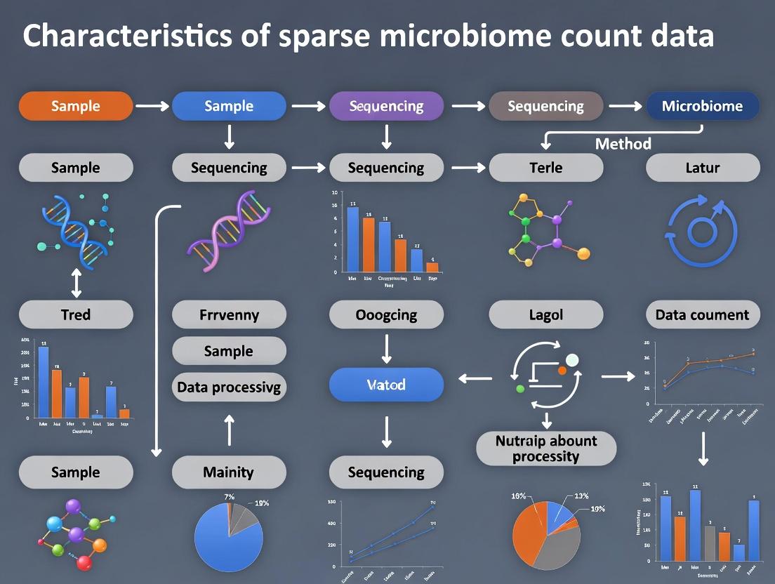
Sparse Microbiome Data Decoded: Key Characteristics, Analytical Challenges, and Advanced Solutions for Biomedical Research

Abstract

This article provides a comprehensive guide to the defining characteristics of sparse microbiome count data, a ubiquitous challenge in modern microbial ecology and biomedical research. It explores the biological and technical origins of sparsity, detailing its impact on statistical analysis and biological inference. The content systematically reviews specialized methodologies for handling zero-inflated distributions, highlights common pitfalls in data preprocessing and analysis, and compares validation strategies for robust model selection. Tailored for researchers and drug development professionals, this resource equips readers with the foundational knowledge and practical framework needed to navigate, analyze, and derive meaningful insights from sparse microbial datasets, ultimately enhancing reproducibility and translational potential in microbiome studies.

Understanding Sparse Microbiome Data: Origins, Characteristics, and Core Analytical Challenges

Within the broader research on the Characteristics of sparse microbiome count data, sparsity is a defining and technically challenging feature. It refers to the overwhelming prevalence of zero counts and taxa with extremely low observed abundances in microbial community sequencing data (e.g., from 16S rRNA or shotgun metagenomics). This sparsity arises from a complex interplay of biological reality (genuine absence or rarity of a microbe in a niche) and technical artifacts (sampling depth, DNA extraction biases, sequencing errors). For researchers, scientists, and drug development professionals, accurately defining, quantifying, and accounting for this sparsity is critical for robust differential abundance testing, biomarker discovery, and ecological inference.

Quantifying Sparsity: Key Metrics and Current Data

Sparsity is typically quantified using several metrics. The following table summarizes these key metrics and their reported ranges from contemporary studies (2022-2024).

Table 1: Quantitative Metrics of Sparsity in Microbiome Data

Metric	Definition	Typical Range in 16S Data	Implications
Overall Zero Proportion	Total zero counts / (Samples × Taxa)	50% - 90%	Direct measure of matrix emptiness; impacts statistical power.
Per-Taxon Zero Prevalence	Proportion of samples where a taxon is absent.	Highly skewed; many taxa are absent in >95% of samples.	Identifies "rare biosphere"; challenges prevalence testing.
Per-Sample Sparsity	Proportion of taxa absent in a single sample.	30% - 80%	Reflects individual heterogeneity and sequencing depth.
Effective Library Size	Sum of counts after normalization (e.g., geometric mean).	Varies widely; low depth increases zero counts.	Normalization is confounded by sparsity.
Singleton/Doubleton Count	Taxa observed exactly 1 or 2 times in entire dataset.	Can represent 20-40% of all observed taxa.	Potential indicator of sequencing errors or ultra-rare taxa.

Source: Consolidated from recent analyses of public repositories like Qiita, MG-RAST, and EMP, and publications in *Nature Methods, Microbiome, and PLOS Computational Biology (2022-2024).*

Experimental Protocols for Investigating Sparsity

Protocol: Controlled Sequencing Depth Experiment to Quantify Technical Zeros

Objective: To dissect the contribution of limited sequencing depth (sampling effort) to observed sparsity.

• Sample Selection: Select a single, homogeneous microbial community standard (e.g., ZymoBIOMICS Microbial Community Standard).
• DNA Extraction & Library Prep: Perform triplicate extractions using a standardized kit (e.g., DNeasy PowerSoil Pro). Prepare one 16S rRNA gene amplicon library (V4 region) using dual-indexed primers.
• High-Depth Sequencing: Sequence the pooled library on an Illumina MiSeq (or NovaSeq) to generate ~5 million paired-end reads per replicate.
• Bioinformatic Processing: Process reads through a standardized pipeline (QIIME 2, DADA2). Denoise, merge, remove chimeras, and assign Amplicon Sequence Variants (ASVs). This yields a "ground-truth" table.
• In Silico Rarefaction: Use a subsampling algorithm (e.g., seqtk) to randomly downsample the high-depth reads from each replicate to decreasing fractions (e.g., 100%, 75%, 50%, 25%, 10%, 5%).
• Sparsity Metric Calculation: For each depth level, recompute the metrics in Table 1. Plot metrics (e.g., Overall Zero Proportion) against sequencing depth.

Protocol: Spike-In Experiment to Detect Genuine vs. Technical Absence

Objective: To differentiate between biological absence and technical dropout.

• Spike-In Preparation: Obtain a known, non-biological synthetic DNA sequence (e.g., External RNA Controls Consortium - ERCC spike-ins) or genomic DNA from a microbe not expected in the host (e.g., Pseudoaheromonas for human gut samples).
• Sample Processing: Spike a consistent, low mass (e.g., 0.1% of total DNA) of the control into aliquots of environmental/biological DNA samples pre-extraction (to assess extraction bias) and post-extraction (to assess PCR/sequencing bias).
• Sequencing & Analysis: Co-sequence spiked samples with unspiked controls. Process data through the same bioinformatics pipeline.
• Detection Analysis: For the known spike-in taxon/sequence, calculate its count across samples. Consistent non-detection in pre-extraction spikes indicates severe technical failure. Variable detection correlates with overall community sequencing efficiency, helping to model "dropout" probability.

Visualizing Concepts and Workflows

Title: Sources Leading to an Observed Zero Count

Title: Core Workflow for Analyzing Sparse Microbiome Data

The Scientist's Toolkit: Key Reagent Solutions

Table 2: Essential Research Reagents & Materials for Sparse Microbiome Research

Item	Function in Sparsity Research	Example Product/Brand
Mock Microbial Community Standards	Provides known composition and abundance to benchmark sparsity and detection limits introduced by wet-lab and computational pipelines.	ZymoBIOMICS Microbial Community Standards, ATCC Mock Microbiome Standards.
External DNA/RNA Spike-Ins	Distinguishes technical zeros (dropouts) from true biological absence. Used to normalize for technical variation.	ERCC RNA Spike-In Mix, Synthetic DNA oligos with unique sequences.
Inhibitor-Removal DNA Extraction Kits	Maximizes DNA yield from low-biomass samples, reducing zeros due to extraction failure.	DNeasy PowerSoil Pro Kit, MagAttract PowerMicrobiome Kit.
High-Fidelity Polymerase for PCR	Reduces PCR amplification bias, preventing under-representation (potential zero inflation) of certain taxa.	Q5 High-Fidelity DNA Polymerase, Phusion Plus PCR Master Mix.
Unique Molecular Identifiers (UMIs)	Tags individual DNA molecules pre-PCR to correct for amplification bias and generate truly quantitative count data.	Duplex-Specific Nuclease-based methods, Commercial UMI kits for amplicon sequencing.
Low-Biomass Positive Controls	Validates entire workflow sensitivity; helps define the "limit of detection" for rare taxa.	Diluted microbial standards, Synthetic cells (e.g., Synthorx).

Within the context of sparse microbiome count data research, distinguishing a biological zero (true absence of a taxon) from a technical zero (failure to detect a present taxon due to methodological limitations) is a fundamental challenge. This distinction is critical for accurate ecological inference, biomarker discovery, and downstream analysis in therapeutic development.

Core Concepts and Definitions

Table 1: Defining Zero Types in Microbiome Data

Zero Type	Definition	Primary Cause	Implications for Analysis
Biological Zero	True absence of a microbial taxon in the sample.	Ecological exclusion, host selection, extreme environmental conditions.	Reflects real biology; can inform on niche specialization or health state.
Technical Zero	Taxon is present but undetected due to methodological limits.	Low biomass, sequencing depth, DNA extraction bias, PCR amplification bias, primer mismatch.	Introduces false negatives; distorts diversity estimates and differential abundance.
Sampling Zero	A subset of technical zero; taxon is present in the environment but not captured in the aliquot.	Finite sampling depth from a heterogeneous mixture.	Leads to under-sampling; can be mitigated by increased sequencing depth.

Quantitative Data on Detection Limits

Source	Typical Impact Range (Estimated % of Zeros)	Key Mitigation Strategy
Sequencing Depth	15-40% of rare taxa in shallow sequencing (<10k reads/sample)	Deep sequencing (>50k reads/sample), rarefaction.
DNA Extraction Bias	Varies by protocol; can be >10-fold difference in recovery	Use of bead-beating, standardized kits (e.g., MoBio PowerSoil).
PCR Amplification Bias	Introduces stochastic variation, especially for low-abundance taxa	Increased PCR replicates, use of modified polymerases.
Primer Mismatch	Taxon-specific; can lead to complete dropout	Use of degenerate primers, multiple primer sets.
Low Biomass Input	Major cause of dropout and increased stochasticity	Minimum input mass protocols, careful contamination controls.

Methodological Framework for Distinction

Experimental Protocol 1: Serial Dilution and Limit of Detection (LoD) Assessment

Purpose: To empirically determine the technical detection limit for specific taxa and protocols.

• Sample Preparation: Spike a known quantity of a control organism (e.g., Pseudomonas aeruginosa) into a sterile matrix or a characterized microbial community.
• Serial Dilution: Create a dilution series spanning 6-8 orders of magnitude (e.g., from 10^6 to 10^0 cells).
• Replicate Processing: Process each dilution point with a minimum of 10 technical replicates through the entire workflow (extraction, amplification, sequencing).
• Data Analysis: For each taxon, model detection probability vs. input abundance. The LoD is defined as the lowest concentration where detection probability is ≥95%.
• Interpretation: Zeros in experimental samples above this LoD for a given taxon are more likely to be biological.

Experimental Protocol 2: Replicate Concordance Analysis

Purpose: To use consistency across technical replicates to infer zero type.

• Experimental Design: Process each biological sample with multiple (n≥5) technical replicates starting from the DNA extraction or PCR step.
• Sequencing & Profiling: Sequence all replicates to a similar depth and generate taxon abundance tables.
• Concordance Scoring: For each taxon-sample pair, calculate the proportion of replicates where it is detected.
• Statistical Modeling: Use a beta-binomial model to estimate the probability of detection given the observed concordance. Low-abundance taxa detected inconsistently are likely technical zeros, while consistent zeros across all replicates suggest a biological zero.

Experimental Protocol 3: Spike-in Control Workflow

Purpose: To normalize for technical variation and infer absolute abundances.

• Control Selection: Introduce known quantities of synthetic or foreign biological spike-in controls (e.g., from the External RNA Control Consortium) prior to DNA extraction.
• Co-processing: Process spike-ins identically with the native sample community.
• Quantification: Measure sequencing yield for each spike-in control.
• Modeling: Construct a recovery curve based on expected vs. observed spike-in reads. Use this model to predict the expected read count for native taxa, given their true abundance. Taxons with observed counts significantly below the predicted detection threshold (e.g., p < 0.01) are candidate biological zeros.

Visualization of Workflows and Relationships

Diagram Title: Framework for Classifying Zeros in Microbiome Data

Diagram Title: Spike-in Controlled Workflow for Zero Inference

The Scientist's Toolkit: Research Reagent Solutions

Table 3: Essential Materials for Zero Characterization Experiments

Item / Reagent	Function & Rationale
Mock Microbial Communities (e.g., ZymoBIOMICS, ATCC MSA-1003)	Defined mixes of known bacterial/fungal strains at characterized ratios. Serves as a ground-truth control for evaluating technical detection limits and biases across the workflow.
External Spike-in Controls (e.g., ERCC RNA Spike-in Mix, SynDNA)	Non-biological or foreign biological sequences added at known concentrations pre-extraction. Enables modeling of technical loss and recovery to differentiate zero types and estimate absolute abundance.
Inhibitor Removal Technology Kits (e.g., MoBio PowerSoil, MagMAX Microbiome)	Critical for low-biomass samples. Removes PCR inhibitors (humics, bile salts) that cause technical zeros by preventing amplification of present taxa.
High-Fidelity DNA Polymerases (e.g., Q5, Phusion)	Reduces PCR-induced technical zeros by offering higher accuracy and lower bias compared to Taq, especially for GC-rich templates.
Degenerate or Broad-Range Primers (e.g., 515F/806R with degeneracy)	Minimizes primer-mismatch-driven technical zeros by accounting for genetic variation in conserved regions (like 16S rRNA gene).
Bead-Beating Lysis Tubes (e.g., Garnet beads, Lysing Matrix E)	Ensures efficient lysis of tough cell walls (e.g., Gram-positives, spores). Prevents technical zeros due to extraction bias.
Library Quantification Kits (e.g., KAPA Library Quant, qPCR)	Accurate quantification of sequencing libraries prevents under-loading, a source of technical zeros due to insufficient sequencing depth.

Statistical and Computational Approaches

Advanced models for zero-inflated count data (e.g., Zero-Inflated Negative Binomial, Hurdle models) are essential. These jointly model the probability of a zero (technical vs. biological process) and the count magnitude (abundance if present). Bayesian frameworks allowing the incorporation of prior knowledge on detection limits (from LoD experiments) are particularly powerful within the thesis of sparse microbiome data research.

Rigorous distinction between biological and technical zeros requires a multi-faceted approach integrating controlled experiments, replicate design, spike-in standards, and specialized statistical models. For researchers in drug development, this distinction is not merely academic; it directly impacts the identification of robust microbial biomarkers and therapeutic targets from inherently sparse data.

In the study of sparse microbiome count data, three statistical properties fundamentally shape analytical approaches: over-dispersion, zero-inflation, and compositionality. These characteristics arise from the nature of amplicon sequence variant (ASV) or operational taxonomic unit (OTU) tables generated via high-throughput sequencing (e.g., 16S rRNA). This guide provides an in-depth technical examination of these properties within the context of advancing microbiome research for therapeutic and diagnostic applications.

Core Statistical Properties: Definitions and Implications

Over-Dispersion

Over-dispersion occurs when the observed variance in count data exceeds the variance predicted by a simple Poisson model, where the mean equals the variance. In microbiome data, this is ubiquitous due to biological heterogeneity, environmental patchiness, and technical noise.

Key Drivers:

• Biological Variation: True microbial abundance variation across samples or habitats.
• Sampling Heterogeneity: Uneven sampling depth and efficiency.
• Model Misspecification: The Poisson assumption is often invalid.

Statistical Models: Negative Binomial (NB) and related distributions are standard for modeling over-dispersed counts.

Zero-Inflation

Zero-inflation refers to an excess of zero counts beyond what is expected under a standard count distribution (e.g., Poisson or Negative Binomial). In microbiome data, zeros are a mixture of:

• Biological Absence: The taxon is genuinely absent from the ecological community.
• Technical Absence: The taxon is present but undetected due to limited sequencing depth (sampling zeros) or methodological artifacts (e.g., PCR dropouts).

Quantitative Impact: Zero counts can constitute 50-90% of entries in a typical OTU/ASV table, severely biasing diversity estimates and differential abundance tests.

Compositionality

Microbiome data is compositional because sequencing yields relative abundance data (counts are constrained by an arbitrary total read count per sample, the library size). Analyses must account for the constant-sum constraint, where an increase in one taxon's relative abundance necessitates an apparent decrease in others.

Core Principle: Data conveys information about relative, not absolute, abundances. Standard Euclidean-based statistics are invalid.

Table 1: Prevalence of Key Properties in Public Microbiome Datasets

Dataset (Reference)	Median % Zeros per Feature	Over-Dispersion Index (Variance/Mean) >1 (%)	Library Size Variation (CV)	Dominant Property
Human Gut (QIITA 13060)	68.5%	92.3%	45.2%	Zero-Inflation
Soil (Earth Microbiome)	81.2%	98.7%	62.1%	Compositionality
Marine (Tara Oceans)	74.8%	95.5%	38.9%	Over-Dispersion
Mock Community	15.1%*	8.4%	10.5%	(Control)

*Primarily due to low abundance and detection limits.

Table 2: Statistical Model Performance Comparison

Model Class	Handles Over-Dispersion?	Handles Zero-Inflation?	Accounts for Compositionality?	Example Algorithm/Package
Standard Poisson GLM	No	No	No	stats::glm
Negative Binomial GLM	Yes	No	No	DESeq2, edgeR
Zero-Inflated Models (ZINB)	Yes	Yes	No	pscl, glmmTMB
ALDEx2 (CLR-based)	Implicitly	Via prior	Yes	ALDEx2
ANCOM-BC	Yes	Robust	Yes	ANCOMBC
Dirichlet-Multinomial	Yes	Implicitly	Yes	MGLM, corncob

Experimental Protocols for Property Assessment

Protocol 1: Diagnosing Over-Dispersion

Objective: Quantify deviation from Poisson expectation. Method:

• Fit a Poisson GLM to count data for a target taxon across samples: log(μ_i) = β_0 + β_1 X_i.
• Extract deviance residuals. For a well-fitting Poisson model, the residual deviance should approximate the degrees of freedom.
• Calculate the dispersion parameter (φ): φ = Residual Deviance / Degrees of Freedom.
• Interpretation: φ ≈ 1 indicates no over-dispersion; φ >> 1 indicates significant over-dispersion. A formal test can be conducted using AER::dispersiontest.

Protocol 2: Quantifying Zero-Inflation

Objective: Test if zeros exceed the expected count from a standard distribution. Method (Vuong Test):

• Fit two models to the same count data: a standard count model (M1: e.g., Negative Binomial) and a zero-inflated version (M2: e.g., ZINB).
• Calculate likelihoods for each observation i under both models: L{M1}(i) and L{M2}(i).
• Compute the likelihood ratio m_i = ln(L{M2}(i) / L{M1}(i)).
• Perform Vuong's non-nested likelihood ratio test on the vector of m_i.
• Interpretation: A significant positive test statistic (p < 0.05) favors the zero-inflated model (M2), confirming zero-inflation.

Protocol 3: Validating Compositional Analysis

Objective: Ensure statistical method is sub-compositionally coherent. Method (Subset Invariance Check):

• Apply your chosen transformation/test (e.g., CLR, ALDEx2) to the full dataset (D_full).
• Randomly select a subset of taxa (e.g., 50%) to create a sub-composition dataset (D_sub).
• Re-apply the same analysis to D_sub.
• Compare the results (e.g., ranks of effect sizes, p-values for shared taxa) between the full and subset analyses.
• Interpretation: Methods that are not compositionally aware will yield inconsistent results between Dfull and Dsub. Robust methods should produce proportional/coherent results.

Visualizations

Title: Analysis Workflow for Sparse Microbiome Data Properties

Title: The Compositionality Challenge in Sequencing Data

The Scientist's Toolkit: Research Reagent Solutions

Table 3: Essential Tools for Analyzing Key Properties

Item/Category	Function in Analysis	Example Product/Software (Reference)
Mock Community Standards	Provides known absolute abundances to benchmark zero-inflation (dropouts) and technical variation.	ATCC MSA-1000: Genomic DNA from 20 bacterial strains. ZymoBIOMICS: Microbial community standards with defined ratios.
Spike-In Controls	Distinguishes biological from technical zeros; aids in estimating absolute abundance from compositional data.	External RNA Controls Consortium (ERCC) spike-ins (for metatranscriptomics). Custom synthetic 16S sequences.
High-Fidelity Polymerase	Reduces PCR amplification bias, a source of technical zero-inflation and over-dispersion.	Q5 High-Fidelity DNA Polymerase (NEB), KAPA HiFi HotStart ReadyMix.
Compositionally-Aware R Packages	Implements statistical models accounting for all three properties.	phyloseq (data handling), ANCOMBC (diff. abundance), microViz (analysis & visualization), corncob (beta-binomial regression).
High-Coverage Sequencing Platform	Reduces sampling zeros by increasing sequencing depth, mitigating one source of zero-inflation.	Illumina NovaSeq 6000, PacBio HiFi long-read sequencing for full-length 16S.
Data Transformation Libraries	Applies log-ratio transforms to address compositionality before downstream analysis.	compositions R package (CLR, ALR, ILR), robCompositions for robust methods.

Impact of Sequencing Depth and Library Size on Observed Sparsity

Thesis Context: This whitepaper is framed within a broader thesis on the Characteristics of Sparse Microbiome Count Data Research. It examines the technical underpinnings of sparsity, a dominant feature of amplicon and shotgun metagenomic sequencing data, focusing on the influence of two fundamental experimental parameters.

In microbiome research, observed sparsity—the prevalence of zero counts in a sample-by-feature (e.g., OTU, ASV, species) matrix—is a statistical property with profound analytical implications. This sparsity arises from both biological (true absence) and technical (undersampling) factors. Sequencing depth (total reads per sample) and library size (the number of uniquely tagged samples pooled in a sequencing run) are primary experimental levers that directly influence the observed sparsity. Understanding their impact is critical for robust experimental design, data interpretation, and downstream statistical analysis.

Core Concepts & Quantitative Relationships

Defining Key Metrics

• Sequencing Depth (D): The number of high-quality sequencing reads assigned to a single sample.
• Library Size (L): The number of individually barcoded samples multiplexed in a single sequencing lane/run.
• Observed Sparsity (S): The proportion of zero entries in a count matrix. Calculated as: S = (Number of Zero Counts) / (Total Number of Matrix Entries).
• Feature Prevalence: The proportion of samples in which a given taxonomic feature is observed.

How Parameters Influence Sparsity

Increased sequencing depth per sample reduces sparsity by detecting low-abundance taxa that would otherwise be missed. However, this relationship is non-linear and subject to diminishing returns. Conversely, for a fixed total number of reads per run, increasing the library size (multiplexing more samples) reduces the depth per sample, thereby increasing observed sparsity.

Table 1: Simulated Impact of Sequencing Parameters on Observed Sparsity

Total Reads Per Run	Library Size (Samples)	Mean Depth Per Sample	Simulated Mean Sparsity (%)	Notes
100 million	20	5 million	~65%	High depth, low sparsity. Rare taxa detected.
100 million	40	2.5 million	~75%	Moderate depth, moderate sparsity.
100 million	100	1 million	~85%	Lower depth, high sparsity. Common taxa only.
50 million	40	1.25 million	~88%	Highlights total run output effect.

Table 2: Empirical Data from Public Studies (16S rRNA Gene Sequencing)

Study Reference	Region	Median Depth	Samples	Reported Sparsity (%)	Key Finding
Costea et al., 2017 (Nature)	V4	50,000	800+	~95%	Sparsity high even at moderate depth; sample heterogeneity dominant.
Schirmer et al., 2015 (Genome Med)	V1-V2	100,000	200	~85%	Depth increases reduced sparsity but plateaus after ~50k reads/sample.

Experimental Protocols for Investigation

In Silico Rarefaction (Subsampling) Analysis

Purpose: To model the effect of varying sequencing depth on observed sparsity using existing data. Methodology:

• Input: A high-depth count matrix from a well-characterized study.
• Subsampling: Randomly subsample (without replacement) each sample's counts to a series of lower depths (e.g., 1k, 5k, 10k, 50k reads).
• Replication: Repeat subsampling 10-100 times per depth level to account for stochasticity.
• Calculation: For each replicate, compute the observed sparsity (S) of the subsampled matrix.
• Visualization: Plot mean S (±SD) against sequencing depth. The curve typically follows a negative exponential decay.

Library Size Dilution Experiment

Purpose: To empirically determine the effect of multiplexing on per-sample depth and sparsity. Methodology:

• Sample Preparation: Use a single, homogeneous microbial community standard (e.g., ZymoBIOMICS Gut Mock Community).
• Library Construction: Prepare 16S rRNA gene amplicon libraries from the same standard. Split into aliquots and apply unique barcode pairs.
• Multiplexing: Create pooled libraries with varying library sizes (e.g., L=12, 24, 48, 96) while keeping the total loading concentration constant.
• Sequencing: Sequence each pooled library on a dedicated MiSeq (or similar) run with the same kit (e.g., v3 600-cycle).
• Bioinformatics: Process all runs through the same DADA2 or QIIME 2 pipeline with identical parameters.
• Analysis: For each run, calculate the mean depth per sample and the observed sparsity of the resulting count matrix. Correlate L with S.

Visualizing the Conceptual and Analytical Workflow

Diagram Title: Trade-off Between Library Size and Sequencing Depth Driving Sparsity

Diagram Title: Computational Workflow for Analyzing Sparsity

The Scientist's Toolkit: Research Reagent Solutions

Table 3: Essential Materials for Investigating Sequencing-Driven Sparsity

Item / Reagent	Function in Sparsity Research	Example Product / Note
Mock Microbial Communities	Provides a ground-truth, defined composition to disentangle technical vs. biological zeros.	ZymoBIOMICS Gut Mock Community, ATCC MSA-2003.
High-Fidelity PCR Polymerase	Minimizes amplification bias and chimera formation, reducing artifactual sparsity.	Q5 Hot Start (NEB), KAPA HiFi.
Unique Dual Index (UDI) Primer Sets	Enables high-level, error-resistant multiplexing (large L) without index crosstalk.	Illumina Nextera XT Index Kit, IDT for Illumina.
Library Quantification Kits	Ensures precise, equimolar pooling of libraries to prevent uneven depth distribution.	Qubit dsDNA HS, KAPA Library Quantification Kit.
PhiX Control v3	Spiked-in during sequencing for quality control and to calibrate low-diversity libraries.	Illumina PhiX Control (1-20% spike-in).
Bioinformatics Pipelines	Standardized processing to ensure sparsity metrics are comparable across studies.	QIIME 2, DADA2, mothur.
Statistical Software Packages	For formal analysis of zero-inflated data and rarefaction curves.	R packages: phyloseq, vegan, ZIMM.

Sequencing depth and library size are inextricably linked in a trade-off that fundamentally shapes the observed sparsity of microbiome data. For a fixed sequencing budget, increasing library size inflates sparsity and may compromise biological conclusions. Researchers must align these parameters with study goals: exploratory studies of diverse communities may prioritize larger library size, while focused studies on low-abundance taxa require greater depth. Standardized reporting of mean depth, library size, and observed sparsity is essential for meta-analyses and reproducibility within the field of sparse microbiome count data research.

This whitepaper addresses a central challenge in modern microbiome research: the analysis of high-dimensional sparse count data where the number of measured taxa (p) vastly exceeds the number of biological samples (n). This p >> n problem is inherent to marker-gene sequencing (e.g., 16S rRNA) and metagenomic shotgun studies, where thousands of microbial features are quantified from tens to hundreds of samples. Framed within a broader thesis on the characteristics of sparse microbiome count data, this guide details the statistical pitfalls, current methodological solutions, and practical experimental protocols for robust analysis.

Core Quantitative Challenge: Data Sparsity and Compositionality

The dimensionality problem is characterized by two intertwined issues: the high-feature, low-sample regime and the compositional nature of the data (relative abundances sum to a constant). The table below summarizes typical dimensions and sparsity levels in contemporary studies.

Table 1: Characteristic Scale of the Dimensionality Problem in Microbiome Studies

Study Type	Typical Sample Size (n)	Typical Features (p)	p/n Ratio	Average Sparsity (% Zero Counts)	Primary Sequencing Platform
16S rRNA (V4 region)	100-500	1,000 - 20,000 ASVs/OTUs	10 - 200	70% - 95%	Illumina MiSeq/NovaSeq
Metagenomic (Shotgun)	50-300	10,000 - 5 Million Genes/MAGs	200 - 100,000	50% - 90%	Illumina NovaSeq
Large Cohort (e.g., AGP)	1,000 - 10,000+	5,000 - 100,000+	5 - 100	60% - 90%	Multiple

Methodological Frameworks and Experimental Protocols

Protocol for Robust Differential Abundance Analysis

Objective: To identify taxa whose abundances are associated with a covariate (e.g., disease state) in high-dimensional, sparse, compositional data.

Reagents & Computational Tools:

• Input Data: ASV/OTU count table, sample metadata.
• Software: R (v4.3+) or Python (v3.10+).
• Key R Packages: phyloseq, DESeq2, edgeR, MaAsLin2, ANCOM-BC, glmnet.
• Key Python Packages: scikit-bio, statsmodels, scikit-learn.

Procedure:

• Pre-filtering: Remove features present in fewer than 10% of samples or with a total count below a threshold (e.g., 20). This reduces p marginally but is critical for noise reduction.
• Normalization: Apply a variance-stabilizing transformation to address compositionality and heteroscedasticity.
  • Option A (Total Sum Scaling): Apply a log-transform after adding a pseudo-count (log1p), followed by center-log-ratio (CLR) transformation.
  • Option B (Reference-Based): Use a robust geometric mean of reference features (e.g., DESeq2's median-of-ratios) or a spike-in standard.
• Modeling: Fit a regularized generalized linear model.
  • For continuous outcomes: Use ridge or elastic-net regression (glmnet) to shrink coefficients of non-informative taxa to zero.
  • For case-control outcomes: Apply a penalized logistic regression or a zero-inflated negative binomial model (edgeR, DESeq2).
• Significance Testing: Apply false discovery rate (FDR, Benjamini-Hochberg) correction to p-values. Report effect sizes (log-fold changes) and confidence intervals.

Protocol for Dimensionality Reduction and Visualization

Objective: To project high-dimensional data into a low-dimensional space for exploration and hypothesis generation.

Procedure:

• Data Transformation: Perform a CLR transformation on the filtered count data to handle compositionality.
• Covariance Estimation: Calculate a robust covariance matrix (e.g., using the corpcor package for shrinkage estimation) to overcome the singularity issue when p > n.
• Principal Components Analysis (PCA): Perform PCA on the robust covariance matrix to obtain principal components (PCs).
• Visualization & Interpretation: Plot samples in the space of the first 2-3 PCs. Color points by metadata. Interpret loadings for the top PCs to identify taxa driving sample separation.

Diagram Title: Dimensionality Reduction & Visualization Workflow

The Scientist's Toolkit: Research Reagent Solutions

Table 2: Essential Materials and Reagents for Addressing the Dimensionality Problem

Item	Function in Addressing Dimensionality	Example Product/Kit
Mock Microbial Community (Even & Staggered)	Serves as a ground-truth control to benchmark statistical models for false positive/negative rates in high-dimensional data.	ZymoBIOMICS Microbial Community Standards
Spike-in Control Standards (External)	Added before DNA extraction to correct for technical variation, enabling absolute abundance estimation and mitigating compositionality effects.	SureQuant Spike-in Mixtures, External RNA Controls Consortium (ERCC) for RNA-seq adapted
High-Fidelity Polymerase & Low-Bias PCR Kits	Reduces amplification bias, minimizing technical zeros and spurious features that inflate dimensionality.	KAPA HiFi HotStart ReadyMix, Q5 High-Fidelity DNA Polymerase
Duplex Sequencing-Compatible Kits	Dramatically reduces sequencing errors, preventing inflation of p due to erroneous unique sequences (ASVs).	Illumina Duplex Sequencing Technology
Bioinformatic Containers/Workflows	Ensures reproducible computational analysis, a prerequisite for validating methods in p >> n scenarios.	QIIME 2, nf-core/mag, Bioconda, Docker/Singularity containers

Advanced Analytical Pathways

The analytical decision-making process for high-dimensional microbiome data involves navigating key trade-offs between model complexity, interpretability, and biological validity.

Diagram Title: Analytical Pathway for High-p, Low-n Data

Table 3: Comparative Analysis of Core Methodological Approaches

Method Category	Specific Technique/Tool	Key Mechanism to Handle p >> n	Best For	Limitations
Differential Abundance	ANCOM-BC	Uses a linear model with bias correction for compositionality; relies on FDR control.	Controlling false positives in relative data.	Conservative; no effect size estimates.
Differential Abundance	DESeq2 / edgeR	Borrows information across features to estimate dispersion; uses regularization priors.	High sensitivity in well-powered studies.	Assumptions can break under extreme sparsity/compositionality.
Regularized Regression	LASSO / Elastic Net	L1/L2 penalty shrinks coefficients of irrelevant taxa to zero, performing feature selection.	Building predictive models; identifying key drivers.	Choice of lambda critical; results can be unstable if n is very low.
Dimensionality Reduction	PhILR Transform + PCA	Phylogenetic Isometric Log-Ratio transform creates orthonormal coordinates before PCA.	Uncorrelated, phylogeny-aware components.	Requires a robust phylogenetic tree.
Network Inference	SPIEC-EASI	Uses sparse inverse covariance estimation (graphical lasso) on CLR data.	Inferring sparse microbial ecological networks.	Very high computational cost; large n required for stability.

Specialized Methods for Sparse Data: From Preprocessing to Advanced Statistical Modeling

Within the broader thesis on the Characteristics of sparse microbiome count data research, the initial steps of data preprocessing and filtering are paramount. Raw amplicon sequencing data is characterized by extreme sparsity, with a high proportion of zeros attributable to both biological absence and technical limitations. This technical guide elucidates the rationale and methodologies for applying prevalence (frequency across samples) and abundance (count level) thresholds, which are critical for distinguishing signal from noise, improving statistical power, and generating biologically interpretable results.

Core Rationale for Filtering

Microbiome count matrices are sparse. Filtering aims to:

• Reduce Noise: Remove low-count taxa likely originating from sequencing errors, index hopping, or laboratory contamination.
• Mitigate Compositional Effects: Alleviate spurious correlations inherent in compositional data by removing non-informative features.
• Enhance Statistical Power: Reduce the multiple testing burden by focusing analyses on taxa with sufficient evidence of presence.
• Improve Computational Efficiency: Decrease dataset dimensions for downstream analyses.

Key Thresholds: Definitions and Quantitative Guidance

Thresholds are typically defined by a minimum abundance (e.g., counts or relative abundance) in a minimum number of samples, defined by prevalence.

Table 1: Common Prevalence & Abundance Thresholds in Literature

Filter Type	Typical Range	Rationale	Commonly Used Value(s)
Prevalence Filter	5% - 30% of samples	Removes taxa that are rarely detected, likely representing transient or spurious signals.	10% (strict) to 20% (lenient)
Abundance Filter	0.001% - 1% Relative Abundance5 - 20 Counts	Removes low-abundance taxa susceptible to technical noise. Often applied as a per-sample floor.	0.01% Rel. Abundance or 10 counts
Total Count Filter	Varies by sequencing depth	Removes entire samples with low total reads, indicative of failed libraries.	e.g., < 1,000 - 10,000 reads
Variance Filter	Top n taxa or percentile	Retains most variable taxa, assuming they are most biologically relevant.	e.g., Top 20% most variable

Detailed Experimental Protocols for Threshold Determination

Protocol 4.1: Systematic Filtering and Alpha/Beta Diversity Assessment

Objective: To empirically determine the impact of different filtering thresholds on core diversity metrics.

• Input: Raw ASV/OTU count table and sample metadata.
• Parameter Sweep: Create a grid of filtering parameters (e.g., prevalence: 5%, 10%, 20%; minimum abundance: 5, 10, 20 counts).
• Application: For each parameter combination, generate a filtered count table.
• Analysis: a. Calculate alpha diversity (e.g., Shannon, Observed Features) for each sample across filtered datasets. b. Calculate beta diversity (e.g., Weighted/Unweighted UniFrac, Bray-Curtis) and perform PERMANOVA to assess sample grouping strength.
• Evaluation: Plot alpha diversity means and variances, and PERMANOVA R² values against filtering stringency. The optimal threshold often balances retention of features against stabilization of diversity metrics.

Protocol 4.2: Positive Control Spike-In Based Threshold Calibration

Objective: To use known, low-abundance spike-in controls to define a minimum abundance threshold for reliable detection.

• Experimental Design: Include a known concentration series of synthetic microbial cells or DNA (e.g., ZymoBIOMICS Spike-in Control) during library preparation.
• Sequencing & Processing: Sequence the sample and process through the standard bioinformatics pipeline up to the count table.
• Detection Analysis: For each spike-in taxon, plot its expected concentration against its observed read count across samples.
• Threshold Setting: Identify the minimum read count at which the lowest concentration spike-ins are consistently detected (e.g., >95% detection rate). This count defines the empirical minimum abundance threshold.

Diagram Title: Microbiome Data Filtering Decision Workflow

The Scientist's Toolkit: Research Reagent Solutions

Table 2: Essential Materials for Filtering & Validation Experiments

Item	Function/Description
ZymoBIOMICS Microbial Community Standard	Defined mock community used to benchmark bioinformatics pipelines, including filtering efficiency and false positive rates.
ZymoBIOMICS Spike-in Control (I)	Low-abundance spike-in control mixed with native samples to empirically set detection limits and abundance thresholds.
PhiX Control v3 (Illumina)	Sequencing run control for error rate calibration; can inform minimum base quality thresholds upstream of abundance filtering.
Qubit dsDNA HS Assay Kit	Fluorometric quantification of library DNA concentration, critical for identifying low-biomass samples prior to total count filtering.
DNeasy PowerSoil Pro Kit (Qiagen)	Standardized soil/pellet DNA extraction kit to minimize batch effects and kit contamination that manifest as low-prevalence noise.
PCR Purification & Clean-up Beads	For consistent amplicon purification, reducing primer dimers that contribute to spurious low-count ASVs.

The choice of thresholds directly influences all subsequent analyses, including differential abundance testing (e.g., DESeq2, edgeR, ANCOM-BC), network construction, and machine learning models. Overly stringent filtering may remove biologically relevant rare taxa, while lenient filtering retains excessive noise. The protocols and rationale outlined herein provide a framework for making informed, reproducible, and study-specific decisions within the challenging context of sparse microbiome data, forming a critical foundation for rigorous research outcomes.

Diagram Title: Downstream Impact of Filtering Thresholds

Within the broader thesis on the Characteristics of Sparse Microbiome Count Data Research, a fundamental statistical challenge is the presence of excess zeros—more than would be expected under standard Poisson or Negative Binomial distributions. This sparsity arises from a combination of biological absence (a taxon is genuinely not present) and technical zeros (a taxon is present but undetected due to sequencing depth or other artifacts). Zero-inflated and hurdle models are two classes of regression models designed to handle this overabundance of zeros, providing more accurate inferences for differential abundance testing, association studies, and community analysis.

Core Model Architectures and Logical Relationships

Diagram Title: Logical Flow of Zero-Inflation vs. Hurdle Processes

Mathematical Formulations

Zero-Inflated Model (e.g., ZINB): The data is modeled as a mixture of a point mass at zero and a count distribution (Negative Binomial). [ P(Y=y) = \begin{cases} \pi + (1-\pi) \cdot \text{NB}(0|\mu, \theta) & \text{if } y=0 \ (1-\pi) \cdot \text{NB}(y|\mu, \theta) & \text{if } y>0 \end{cases} ] Where (\pi) is the probability of a structural zero from the Bernoulli process, (\mu) is the mean of the count distribution, and (\theta) is the dispersion parameter.

Hurdle Model (e.g., Negative Binomial Hurdle): The model uses one process for the zero vs. non-zero decision and a separate, truncated process for positive counts. [ P(Y=y) = \begin{cases} \pi & \text{if } y=0 \ (1-\pi) \cdot \frac{\text{NB}(y|\mu, \theta)}{1 - \text{NB}(0|\mu, \theta)} & \text{if } y>0 \end{cases} ]

Quantitative Model Comparison

Table 1: Key Characteristics of Zero-Inflated vs. Hurdle Models for Microbiome Data

Feature	Zero-Inflated Models (ZIP/ZINB)	Hurdle Models (PH/NBH)
Conceptual View	Two processes: one generates only zeros, the other generates counts (which may be zero).	Two sequential parts: a hurdle (zero vs. non-zero) and a truncated count model.
Source of Zeros	Two types: "structural" (from point mass) and "sampling" (from count model).	One type: all zeros from the hurdle component.
Interpretation	Distinguishes between "always zero" and "sometimes zero" taxa.	Distinguishes between "presence" and "abundance given presence".
Parameterization	Mixture model: Bernoulli (logit) for zero-inflation + Poisson/NB (log) for counts.	Two separate models: Bernoulli (logit) for hurdle + Zero-Truncated Poisson/NB (log) for counts.
Ideal Use Case	When a subpopulation is never expected to have the taxon (e.g., non-colonized host).	When the mechanisms for presence/absence and level of abundance are distinct.
Common R Packages	pscl, GLMMadaptive, zinbwave	pscl, countreg

Experimental Protocol for Model Application in Microbiome Analysis

Protocol Title: Differential Abundance Analysis of Sparse 16S rRNA Amplicon Data Using Hurdle and Zero-Inflated Models.

1. Data Preprocessing & Exploration:

• Input: Raw OTU/ASV count table, sample metadata.
• Steps: a. Perform quality control, normalization (e.g., CSS, TSS, or use model offsets for sequencing depth). b. Exploratory analysis: Calculate mean, variance, and percentage of zeros per taxon. c. Split data into training (≥70%) and validation sets.

2. Model Fitting & Selection:

• Candidate Models: Fit standard Negative Binomial (NB), Zero-Inflated Negative Binomial (ZINB), and Negative Binomial Hurdle (NBH) models for each taxon of interest.
• Covariates: Include biological conditions of interest (e.g., disease state, treatment) and relevant confounders (e.g., age, batch) in both the count and zero-inflation/hurdle components.
• Code Example (R pscl package):

3. Model Diagnostics & Validation:

• Goodness-of-Fit: Compare models using AIC/BIC and Likelihood Ratio Tests (LRT).
• Residual Checks: Use randomized quantile residuals to assess overall fit.
• Zero Prediction: Evaluate the model's ability to predict the observed number of zeros.
• Cross-Validation: Assess out-of-sample prediction error on the hold-out validation set.

4. Inference & Interpretation:

• Extract coefficients and p-values (or Bayesian credible intervals) for the covariate of interest from both the count component (affecting abundance) and the zero component (affecting presence/absence).
• Report results separately for each process (e.g., "Treatment was associated with a significant increase in the odds of taxon X being present (hurdle log-odds = Y, p < 0.01) and, conditional on presence, a significant increase in its abundance (log-fold change = Z, p < 0.05).").

Diagram Title: Microbiome Differential Abundance Analysis Workflow

The Scientist's Toolkit: Research Reagent Solutions

Table 2: Essential Tools for Analyzing Sparse Count Data with Zero-Inflated and Hurdle Models

Tool/Reagent	Function in Analysis	Example/Note
Statistical Software (R/Python)	Primary environment for model fitting, testing, and visualization.	R with pscl, glmmTMB, MAST packages. Python with statsmodels, scikit-learn.
High-Performance Computing (HPC)	Enables fitting complex, computationally intensive models to large OTU tables.	Slurm cluster for parallel processing across hundreds of taxa.
Normalized Count Matrix	Corrects for variable sequencing depth, used as the primary input data.	Generated via metagenomeSeq (CSS), DESeq2 (median of ratios), or total sum scaling (TSS).
Model Diagnostic Plots	Visual tools to assess model fit and identify violations of assumptions.	Rootogram, QQ plot of randomized quantile residuals, fitted vs. observed zeros plot.
Likelihood Ratio Test (LRT)	Formal statistical test to compare nested models (e.g., NB vs. ZINB).	Determines if the zero-inflation component is statistically warranted.
AIC / BIC Criteria	Metrics for model selection among non-nested or multiple candidate models.	Used to choose between ZINB and NBH for a given taxon.
Bayesian Frameworks (Stan)	Alternative for flexible model specification and obtaining full posterior distributions.	Implemented via R brms package for robust hierarchical ZINB models.

Microbiome count data derived from high-throughput sequencing is intrinsically compositional. The data consists of relative abundances constrained to a constant sum, making absolute quantitation impossible without external reference. This characteristic is profoundly exacerbated by sparsity—an abundance of zeros due to biological absence, under-sampling, or technical dropout. Research within the thesis on Characteristics of sparse microbiome count data must therefore employ statistical methods grounded in Compositional Data Analysis (CoDA) principles to avoid erroneous conclusions. This guide details two leading CoDA-based methods: ALDEx2 and ANCOM-BC, providing protocols, visualizations, and a toolkit for their application.

Core Principles and Method Comparison

Both ALDEx2 and ANCOM-BC address compositionality and sparsity but through distinct philosophical and technical approaches.

Table 1: Comparison of ALDEx2 and ANCOM-BC

Feature	ALDEx2	ANCOM-BC
Core Principle	Monte Carlo sampling from a Dirichlet distribution to generate posterior probability distributions of relative abundances.	Log-ratio linear modeling with bias correction for sample-specific sampling fractions and sparse data.
Handling of Zeros	Uses a uniform prior, equivalent to adding a small pseudo-count proportional to feature prevalence.	Employs a carefully designed pseudo-count strategy to mitigate false positives from log-ratios involving zeros.
Hypothesis Test	Tests for difference in within-condition dispersion and difference in central tendency (median). Uses Benjamini-Hochberg FDR.	Tests the null hypothesis that the log-fold change is zero. Uses a multi-step procedure to control FDR.
Output	Effect size (median difference between groups) and expected P-value/FDR.	Log-fold change estimate, standard error, W-statistic, and adjusted P-value.
Key Assumption	Features are not highly correlated. Data can be adequately modeled via Dirichlet Monte Carlo.	The sampling fraction is constant across features within a sample. Most features are not differentially abundant.
Strengths	Robust to uneven sampling depth, identifies both differential abundance and dispersion.	Provides unbiased log-fold change estimates, good control of Type I error.
Limitations	Computationally intensive for very large datasets. Effect size is relative, not absolute.	Can be conservative; model assumptions may be violated in complex communities.

Detailed Experimental Protocols

Protocol 1: Differential Abundance Analysis with ALDEx2

Input: A count table (features x samples) and a sample metadata table with group identifiers.

• Installation and Loading: In R, install BiocManager and then ALDEx2.

• Data Preprocessing: Ensure count table contains only integers. No rarefaction or normalization is required.

• Generate Monte-Carlo Instances: Use aldex.clr() to create n (typically 128 or 256) Dirichlet Monte Carlo instances of the center-log-ratio (CLR) transformed data.

• Calculate Test Statistics: Perform Welch's t-test and Wilcoxon rank test on the Monte Carlo instances using aldex.ttest().

• Compute Effect Sizes: Calculate effect sizes (median difference in CLR values) using aldex.effect().

• Combine Results and Interpret: Merge outputs. Features with both a low FDR (e.g., < 0.1) and a meaningful effect size (e.g., |effect| > 1) are considered significant.

Protocol 2: Differential Abundance Analysis with ANCOM-BC

Input: A count table and sample metadata, potentially with a sample_var (sample ID) and group_var.

• Installation and Loading: Install and load the ANCOMBC package.

• Data Structuring: Format data as a phyloseq object or ensure matrices are correctly oriented.

• Run Primary Analysis: Execute the ancombc2() function, specifying the formula and grouping variable.

• Extract and Interpret Results: The output is a list. The res element contains the main results dataframe.

Visualization of Workflows and Relationships

Diagram Title: ALDEx2 Analysis Workflow

Diagram Title: ANCOM-BC Bias Correction Principle

Diagram Title: Guide to Choosing ALDEx2 vs ANCOM-BC

The Scientist's Toolkit: Research Reagent Solutions

Table 2: Essential Reagents and Materials for CoDA-Based Microbiome Analysis

Item / Reagent	Function / Purpose	Example / Notes
High-Fidelity DNA Polymerase	Amplification of 16S rRNA gene regions for sequencing with minimal bias.	KAPA HiFi HotStart ReadyMix – Reduces PCR artifacts and chimeras.
Mock Microbial Community (Standard)	Validation of experimental and bioinformatic pipeline, quantifying technical variance.	ZymoBIOMICS Microbial Community Standard – Defined composition of known bacterial strains.
Quant-iT PicoGreen dsDNA Assay	Accurate fluorometric quantification of dsDNA library concentrations before sequencing.	Ensures balanced loading across sequencing lanes.
AMPure XP Beads	Solid-phase reversible immobilization (SPRI) for post-PCR library clean-up and size selection.	Critical for removing primer dimers and optimizing library fragment size.
Unique Dual-Index Primers	Multiplexing samples on a sequencing run while minimizing index hopping.	Nextera XT Index Kit v2 or Illumina IDT for Illumina kits.
Positive Control Spike-in (Sequencing)	Monitoring for batch effects and compositionality in the final sequence data.	External RNA Controls Consortium (ERCC) spike-ins for RNA-seq; synthetic 16S constructs for microbiome.
R/Bioconductor Packages	Software implementation of CoDA methods and associated data handling.	ALDEx2, ANCOMBC, phyloseq, MicrobiomeStat, zCompositions.
High-Performance Computing (HPC) Resources	Enables Monte Carlo simulations and large-scale linear modeling.	Access to clusters with sufficient RAM (≥32 GB) and multi-core processors.

Regularization Techniques (e.g., LASSO) for High-Dimensional, Sparse Feature Selection

The analysis of sparse microbiome count data presents a quintessential high-dimensional problem. In a typical 16S rRNA gene sequencing study, the number of features (Operational Taxonomic Units, OTUs) often vastly exceeds the number of samples (n << p). This data is characterized by extreme sparsity, with a majority of counts being zero due to biological absence or undersampling, over-dispersion, and compositionality. Within the broader thesis on "Characteristics of sparse microbiome count data research," regularization techniques like LASSO (Least Absolute Shrinkage and Selection Operator) are not merely statistical tools but essential frameworks for robust feature selection, model stability, and biological interpretability. This guide details their application, addressing the unique challenges of microbiome datasets.

Core Regularization Techniques: Theory and Application

Regularization introduces a penalty term to a loss function to constrain model complexity, preventing overfitting and performing implicit feature selection in high-dimensional settings.

Table 1: Comparison of Key Regularization Techniques for Sparse Data

Technique	Penalty Term (Ω(β))	Key Property	Microbiome Application Pros	Microbiome Application Cons
LASSO (L1)	λ∑⎮βⱼ⎮	Sparse solutions, feature selection.	Directly selects discriminative taxa; handles p >> n.	Tends to select only one from a correlated group; unstable with high correlation.
Ridge (L2)	λ∑βⱼ²	Shrinks coefficients, no selection.	Stable with correlated features; good for prediction.	Retains all features, limiting interpretability in high-dimensions.
Elastic Net	λ₁∑⎮βⱼ⎮ + λ₂∑βⱼ²	Hybrid of L1 and L2.	Selects groups of correlated taxa; more stable than pure LASSO.	Two hyperparameters (λ₁, λ₂) to tune.
Adaptive LASSO	λ∑ wⱼ⎮βⱼ⎮	Weighted L1 penalty.	Can achieve oracle properties; consistent variable selection.	Requires initial consistent estimator (e.g., Ridge) for weights.
Zero-Inflated Models	Penalty on count model (e.g., ZINB)	Accounts for excess zeros.	Explicitly models structural zeros; biologically interpretable for microbiome.	Computationally intensive; complex likelihood.

For microbiome counts, the penalized loss function is often applied to a negative binomial or zero-inflated negative binomial regression to handle over-dispersion and excess zeros:

[ \text{Loss}(β) = -\text{Log-Likelihood}(y | X, β) + \lambda \cdot \Omega(β) ]

Experimental Protocols for Microbiome Applications

Protocol 3.1: Baseline LASSO-Penalized Logistic Regression for Case-Control Studies

Objective: To identify a minimal set of microbial taxa predictive of a binary outcome (e.g., disease vs. healthy).

• Data Preprocessing:

  • Input: Raw OTU or ASV count table.
  • Filtering: Remove taxa with prevalence < 10% across samples.
  • Normalization: Convert counts to Centered Log-Ratio (CLR) or relative abundance. For counts, use a variance-stabilizing transformation.
  • Covariates: Standardize all continuous features (mean=0, sd=1).

• Model Fitting:

  • Use glmnet (R) or sklearn.linear_model.LogisticRegression (Python) with penalty='l1'.
  • Perform k-fold cross-validation (k=5 or 10) on the training set to select the optimal lambda (λ) that minimizes the deviance or misclassification error.

• Feature Selection & Validation:

  • Extract non-zero coefficients at the optimal λ.
  • Apply the selected features and the λ to the held-out test set for performance evaluation (AUC, accuracy).
  • Perform stability analysis via bootstrap or subsampling to assess feature selection reliability.

Protocol 3.2: Penalized Zero-Inflated Negative Binomial Regression for Quantitative Traits

Objective: To model sparse count data with excess zeros while selecting features associated with a continuous outcome.

• Data Preprocessing: Similar to Protocol 3.1, but retain count nature. Use a filtering threshold based on both prevalence and total abundance.

• Model Fitting:

  • Use the pscl (R) package for zero-inflated models or zeroinfl from statsmodels (Python).
  • Implement a coordinate descent algorithm with a LASSO penalty on the count component's coefficients.
  • Optimize both the zero-inflation and count model parameters simultaneously with a combined penalty parameter.

• Analysis:

  • Distinguish between "structural zeros" (modeled by the zero-inflation component) and "sampling zeros" (modeled by the count component).
  • Report selected taxa from the count model and their incident rate ratios (exponentiated coefficients).

Visualizations

Title: LASSO Feature Selection Workflow for Microbiome Data

Title: Effect of Different Regularization Penalties

The Scientist's Toolkit: Research Reagent Solutions

Table 2: Essential Tools for Regularized Analysis of Microbiome Data

Item/Category	Specific Tool or Package	Function & Relevance
Primary Analysis Software	R (v4.3+) with phyloseq, microbiome packages	Container for OTU table, taxonomy, sample metadata. Essential for preprocessing and exploration.
Penalized Regression Engine	glmnet (R), sklearn.linear_model (Python)	Efficiently fits LASSO, Ridge, Elastic Net models via coordinate descent for generalized linear models.
High-Performance Computing	High-memory compute cluster or cloud (AWS, GCP)	Necessary for bootstrapping stability analysis and cross-validation on large datasets.
Specialized Count Models	corncob (R), statsmodels (Python)	Implements beta-binomial and related models for differential abundance with regularization options.
Model Tuning & Validation	tidymodels (R), mlr3 (R), or scikit-learn pipelines	Streamlines cross-validation, hyperparameter grid search, and performance metric calculation.
Visualization & Reporting	ggplot2 (R), matplotlib/Seaborn (Python), ComplexHeatmap (R)	Creates coefficient paths, AUC curves, and heatmaps of selected features across samples.
Stability Selection Package	stabs (R) or custom bootstrap scripts	Quantifies the reliability of feature selection under data perturbation.
Data Transformation Library	compositions (R) for CLR, DESeq2 for VST	Provides robust transformations for compositional microbiome data before penalized regression.

Utilizing Phylogenetic Information and Tree-Based Methods to Leverage Sparsity

Research into microbial communities via high-throughput sequencing generates sparse count matrices. This sparsity—a high proportion of zeros due to biological absence, under-sampling, or technical limitations—is a fundamental characteristic that complicates statistical analysis. Within this thesis, we posit that leveraging the innate phylogenetic structure of microbial data is paramount for transforming sparsity from an analytical hurdle into a source of biological insight. Phylogenetic trees encode evolutionary relationships, providing a structured correlation metric between microbial taxa. This guide details how integrating this information with sophisticated tree-based statistical methods enhances signal detection, improves prediction accuracy, and yields more biologically interpretable models in the face of extreme data sparsity.

Core Methodologies and Quantitative Summaries

Phylogenetically Informed Sparsity Techniques

Table 1: Comparison of Phylogenetic Regularization Methods for Sparse Data

Method	Core Mechanism	Sparsity Type Addressed	Key Hyperparameter	Implementation (R/Python)
Phylogenetic LASSO	L1 penalty on phylogenetically transformed coefficients	Structured (clade-level)	Regularization λ	glasso (R), custom CV
Phylogenetic Elastic Net	Combined L1 & L2 penalties on phylogenetic contrasts	Structured & Grouped	λ, α mixing parameter	glmnet with contrasts
Phylogenetic Factor Analysis	Latent factors constrained by tree covariance	Low-rank approximation	Number of factors (k)	phylofactor (R)
Tree-Guided Group LASSO	L2 penalty per clade, then L1 across clades	Hierarchical Group	Group regularization weights	gglasso (R)
UniFrac-weighted Regression	Penalization weighted by phylogenetic distance	Distance-based	Distance decay parameter	Custom optimization

Experimental Protocol: Phylogenetic LASSO for Disease Association

Aim: Identify microbial clades associated with a binary disease outcome from sparse 16S rRNA gene sequencing data.

Protocol Steps:

• Data Input: OTU/ASV count table (m samples x n taxa), rooted phylogenetic tree, sample metadata with outcome.
• Preprocessing: Convert counts to relative abundance or use a variance-stabilizing transformation for counts (e.g., DESeq2). Center-log-ratio (CLR) transformation is common.
• Phylogenetic Contrasts: Compute phylogenetically independent contrasts (PIC) or use the phylogenetic incidence matrix (from ape::vcv.phylo) to create a transformation matrix P.
• Model Formulation: Let y be the outcome vector and Z the transformed abundance matrix (Z = X P). Solve: min(||y - Zβ||² + λ||β||₁), where β are coefficients in the phylogenetically transformed space.
• Regularization Path: Use 10-fold cross-validation repeated 3 times over a sequence of λ values to select the optimal λ that minimizes prediction error (MSE or deviance).
• Back-Transformation: Transform significant β coefficients back to the original taxonomic space via P⁻¹ for biological interpretation, identifying entire clades rather than individual taxa.
• Validation: Assess model performance on a held-out test set using AUC-ROC (for classification) or RMSE (for regression). Compare against a non-phylogenetic LASSO baseline.

Tree-Based Machine Learning Methods

Table 2: Performance of Tree-Based Models on Sparse Microbiome Data

Model Class	Example Algorithm	Handles Sparsity via Phylogeny?	Key Advantage for Sparse Data	Typical Performance Gain (AUC Increase vs. Baseline)*
Decision Trees	CART	No (uses raw features)	Non-parametric, handles zeros	+0.02 - +0.05
Random Forest	ranger, randomForest	Possible via partitioned data	Reduces overfitting, impurity measures	+0.03 - +0.07
Gradient Boosting	XGBoost, LightGBM	Can incorporate tree as constraint	Iterative correction, high accuracy	+0.05 - +0.10
Phylogenetic RF	phyloseq + custom	Yes (uses UniFrac distances)	Directly incorporates lineage	+0.08 - +0.15
Tree-Structured NN	Custom architecture	Yes (as a prior in the network)	Captures complex non-linear patterns	+0.10 - +0.18

*Performance gain is illustrative, based on simulated and benchmark studies (e.g., soil vs. gut microbiome prediction tasks).

Mandatory Visualizations

Diagram Title: Phylogenetic Regularization Workflow for Sparse Microbiome Data

Diagram Title: Phylogenetic Tree-Based Machine Learning Approaches

The Scientist's Toolkit: Research Reagent Solutions

Table 3: Essential Tools for Phylogenetically Informed Sparse Data Analysis

Category	Item/Software	Function in Analysis	Key Consideration for Sparsity
Bioinformatics	QIIME2, DADA2, mothur	Processes raw sequences into ASV/OTU tables and constructs/deblurs phylogenetic trees.	Pipeline choice impacts zero-inflation (DADA2→more zeros, OTU clustering→fewer).
Phylogenetic Tool	ape (R), ETE3 (Python), FastTree	Core libraries for tree manipulation, distance calculation (UniFrac), and contrast computation.	Ensure tree is rooted and includes all taxa in count matrix, even rare ones.
Statistical Engine	glmnet, phyloseq, mixOmics (R), scikit-learn (Python)	Provides optimized routines for regularized regression, data integration, and machine learning.	Check handling of excessive zeros; CLR transformation requires pseudocounts.
Specialized R Packages	phylolm, phylofactor, gglasso, siamese	Implements phylogenetic regression, factorization, and group-lasso directly.	Critical for modeling sparse, tree-structured coefficients.
Visualization	ggtree, phyloseq Plot, GraPhlAn	Creates publication-ready figures of tree-annotated results and clade associations.	Highlighting significant clades, not individual sparse taxa, improves interpretation.
Benchmark Dataset	American Gut Project, TARA Oceans, Human Microbiome Project	Publicly available, well-characterized sparse datasets for method validation.	Sparsity patterns differ by body site/environment; test generalizability.

Navigating Pitfalls and Optimizing Analysis of Sparse Microbiome Datasets

Modern microbiome research generates high-throughput sequencing data characterized by extreme sparsity, compositionality, and over-dispersion. These inherent characteristics violate the core assumptions of traditional parametric models derived from Gaussian distributions and the Pearson correlation coefficient. This whitepaper details the technical pitfalls of applying these inappropriate methods and provides validated alternatives.

Fundamental Data Characteristics and Model Assumption Violations

Microbiome count data from 16S rRNA or shotgun metagenomic sequencing exhibits specific properties that conflict with Gaussian and Pearson frameworks.

Table 1: Characteristics of Microbiome Count Data vs. Gaussian/Pearson Assumptions

Data Characteristic	Description	Violated Assumption	Consequence of Misapplication
Compositionality	Data sum to a fixed total (library size); only relative abundances are meaningful.	Independence of observations.	Spurious correlations; false positive/negative associations.
Zero-Inflation	High frequency of zero counts (technical & biological).	Continuity, normality.	Biased mean/variance estimates; invalid p-values.
Over-Dispersion	Variance > Mean (Negative Binomial distribution).	Homoscedasticity (equal variance).	Underestimated error; inflated type I error.
Non-Normality	Discrete, skewed, non-negative counts.	Normal distribution of errors/residuals.	Invalid inference, poor model fit.
High-Dimensionality	Features (taxa) >> Samples (n).	Full rank covariance matrix.	Singular matrix; correlation cannot be computed.

The Pearson Correlation Pitfall in Microbial Association Networks

Using Pearson correlation on raw or transformed relative abundance data is a prevalent error.

Experimental Protocol: Benchmarking Correlation Metrics

• Objective: Compare the false positive rate (FPR) of Pearson vs. compositionally-aware methods in detecting microbial associations from simulated count data.
• Data Simulation: Using the SPIEC-EASI or seqtime R package, generate synthetic microbial count matrices with known ground-truth interaction networks (e.g., 200 taxa, 100 samples). Incorporate realistic sparsity (70-90% zeros) and compositionality.
• Methods Applied:
  • Naïve Approach: Calculate Pearson correlation on CLR-transformed counts.
  • Compositional Approach: Calculate SparCC or proportionality (e.g., rho).
  • Model-Based Approach: Fit a graphical model via SPIEC-EASI (MB).
• Evaluation: Compute Precision-Recall curves and FPR against the known network. Area Under the Curve (AUC) is the primary metric.

Table 2: Performance of Correlation Methods on Sparse Count Data (Simulated)

Method	AUC (Precision-Recall)	False Positive Rate (%)	Runtime (s)	Compositionally Aware?
Pearson (on CLR)	0.31 ± 0.04	42.7 ± 5.1	1.2	No
SparCC	0.78 ± 0.03	8.3 ± 2.4	15.7	Yes
SPIEC-EASI (MB)	0.85 ± 0.02	5.1 ± 1.8	122.5	Yes

Diagram 1: Correlation Analysis Pathways for Microbiome Data

Misapplication of Gaussian-Based Linear Models

Using linear regression, ANOVA, or other Gaussian-based models on count data without proper specification leads to biased inference.

Experimental Protocol: Differential Abundance Analysis Comparison

• Objective: Evaluate Type I error control in differential abundance testing between two sample groups.
• Data: Use a curated public dataset (e.g., from IBDMDB) with a balanced case-control design. Introduce a set of non-differentially abundant "null" taxa via permutation.
• Methods Tested:
  • Mistaken Approach: Linear model (LM) on arcsin-sqrt or log-transformed proportions.
  • Standard Count Regression: Negative Binomial model (e.g., DESeq2, edgeR).
  • Compositional Model: ALDEx2 (CLR + Wilcoxon) or ANCOM-BC.
• Evaluation: For the permuted "null" taxa, calculate the empirical Type I error rate (proportion of p-values < 0.05). The expected rate is 5%.

Table 3: Type I Error Rates in Differential Abundance Testing

Modeling Method	Underlying Distribution	Avg. Type I Error Rate (%)	Handles Compositionality?
LM on Log-Proportions	Gaussian (Incorrect)	18.9	No
Negative Binomial (DESeq2)	Negative Binomial	5.2	Partial (via Size Factors)
ALDEx2 (CLR + Wilcoxon)	Dirichlet-Multinomial	4.8	Yes
ANCOM-BC	Linear Model with BC	5.1	Yes

Diagram 2: Model Selection for Differential Abundance Analysis

The Scientist's Toolkit: Essential Research Reagent Solutions

Table 4: Key Analytical Tools for Sparse Microbiome Data

Tool/Reagent	Category	Function & Purpose	Key Consideration
DESeq2 / edgeR	Differential Abundance R Package	Models raw counts using negative binomial GLM; robust to library size differences.	Not inherently compositional; requires careful experimental design.
ANCOM-BC	Differential Abundance R Package	Addresses compositionality via a linear model with bias correction.	Controls FDR well; provides log-fold-change estimates.
ALDEx2	Differential Abundance R Package	Uses Dirichlet-multinomial simulations & CLR transformation; compositional.	Output is centered log-ratio values; uses non-parametric tests.
SPIEC-EASI	Network Inference R Package	Infers microbial ecological networks from compositional data.	Computationally intensive; combines data transformation and graphical model selection.
SparCC / propr	Correlation Metric	Estimates correlation/sparsity for compositional data (e.g., proportionality).	Faster than model-based networks but less powerful for complex dependencies.
Phyloseq	Data Handling R Package	Unified data structure and basic analysis for microbiome census data.	Essential for preprocessing, visualization, and piping data to other tools.
ZINB / Hurdle Models	Statistical Model	Explicitly models zero-inflation with a two-component mixture model.	Crucial for datasets where biological zeros are suspected (e.g., rare taxa).
QIIME 2 / DADA2	Pipeline	Processes raw sequences into Amplicon Sequence Variant (ASV) tables.	Generates the foundational count table; choice affects downstream sparsity.
Greengenes / SILVA	Reference Database	Provides taxonomic classification for 16S rRNA sequence variants.	Database choice and version influence taxonomic assignment and analysis.

Alpha-diversity estimates, quantifying the microbial diversity within a single sample, are foundational to microbiome research. However, the inherent sparsity and uneven sequencing depth of microbiome count data introduce significant biases into these metrics. This technical guide, framed within a broader thesis on the characteristics of sparse microbiome count data, examines the sources of bias in common richness estimators and rarefaction procedures, and presents current methodologies for obtaining robust, comparable alpha-diversity estimates.

Core Challenges & Quantitative Comparisons

The primary challenge stems from the compositional nature of sequencing data, where observed counts are relative and subject to library size variation. Traditional rarefaction (subsampling to an even depth) discards valid data, while uncorrected richness metrics (e.g., observed ASVs) are highly sensitive to sampling depth.

Table 1: Comparison of Alpha-Diversity Estimation Methods & Their Biases

Method	Principle	Key Bias/Assumption	Sensitivity to Sparsity	Data Usage
Observed Richness (S_obs)	Count of distinct features.	Heavily underestimates true richness; highly sensitive to sequencing depth.	Very High	All data, but incomplete.
Traditional Rarefaction	Subsample to equal depth.	Introduces variance; discards data; assumes discarded reads are random.	High (post-subsampling)	Partial (only subsample).
Chao1	Non-parametric estimator based on singletons/doubletons.	Assumes rare taxa inform unobserved ones; underestimates for highly uneven communities.	Moderate-High	All data.
ACE (Abundance-based Coverage Estimator)	Estimates richness based on taxa with abundance ≤10.	Biased when high-frequency singletons exist; performs poorly with extreme unevenness.	Moderate	All data.
Shannon (log-based) / Simpson (dominance)	Evenness-weighted indices.	Less sensitive to rare taxa than richness; but still influenced by depth.	Low-Moderate	All data.
Rarefaction with Extrapolation (iNEXT)	Uses observed data to predict diversity at a standardized depth or via extrapolation.	Relies on asymptotic models; interpolation reliable, extrapolation requires caution.	Low	All data (modeled).
Bias-Corrected Chao1 (Chao1-bc)	Adjusts for singleton bias.	Reduces bias from singleton inflation in sparse data.	Moderate	All data.
Phylogenetic Diversity (Faith's PD)	Sum of branch lengths in phylogenetic tree.	Sensitive to tree construction and missing taxa due to depth.	High	All data + phylogeny.

Detailed Experimental Protocols

Protocol 3.1: Evaluating Bias via In-Silico Dilution

Objective: To quantify the sensitivity of alpha-diversity metrics to sequencing depth using real data.

• Data Selection: Start with a deep-sequenced microbiome dataset (e.g., from a mock community or a deeply sequenced environmental sample).
• Creation of Sparse Datasets: Programmatically subsample (without replacement) the count data from the original library size (N) to progressively smaller fractions (e.g., 90%, 75%, 50%, 25%, 10% of N). Repeat this subsampling 100 times at each depth to capture variance.
• Metric Calculation: For each subsampled dataset, calculate a suite of alpha-diversity metrics: Observed Richness, Chao1, Shannon, Simpson, and Faith's PD (if phylogeny available).
• Bias Calculation: For each metric at each depth, compute the percentage deviation from the metric's value calculated on the full-depth (N) dataset. Plot mean deviation and confidence intervals against sequencing depth.

Protocol 3.2: Comparing Rarefaction vs. Extrapolation with iNEXT

Objective: To standardize diversity comparisons using a robust statistical framework.

• Data Input: Prepare an OTU/ASV table (samples x features) with absolute counts. Do not transform to relative abundance.
• Software Implementation: Utilize the iNEXT R package (interface for INterpolation/EXTrapolation).
• Standardization: Run iNEXT() on the entire dataset, specifying the diversity order q=0 (richness), q=1 (Shannon exponential), and q=2 (Simpson inverse). Set a standardized comparison depth—typically the double of the minimum sample size or a predefined "coverage" value (e.g., 97% sample completeness).
• Output & Analysis: The function outputs estimates (with confidence intervals) for each sample at the standardized depth, derived from interpolation (for depths less than the original) or extrapolation (for greater depths, but capped at double the reference sample size). Compare these standardized estimates across sample groups using appropriate statistical tests (e.g., Kruskal-Wallis).

Protocol 3.3: Assessing Estimator Performance with Mock Communities

Objective: To validate richness estimators against a known ground truth.

• Mock Community Data: Obtain sequencing data from a defined mock community (e.g., ZymoBIOMICS, Bee Gut Mock) where the true number of constituent strains/species is known.
• Processing: Process raw sequences through the same bioinformatics pipeline (DADA2, QIIME2, mothur) as experimental samples to generate an ASV/OTU table.
• Calculation & Comparison: Calculate Observed Richness, Chao1, ACE, and Bias-Corrected Chao1 for each technical replicate of the mock community.
• Performance Metric: Compute the mean absolute error (MAE) and bias (mean deviation from true known richness) for each estimator across replicates. The estimator with the lowest MAE and bias for the given data type is preferable.

Visualization of Method Selection & Workflow

(Diagram Title: Alpha-Diversity Estimation Decision Workflow)

The Scientist's Toolkit: Research Reagent Solutions

Table 2: Essential Materials & Tools for Alpha-Diversity Analysis

Item	Function in Analysis	Example/Note
Mock Community Standards	Ground truth for validating bioinformatics pipelines and richness estimators.	ZymoBIOMICS Microbial Community Standards; ATSA Mock Communities.
High-Fidelity Polymerase	Critical for reducing PCR amplification bias prior to sequencing, impacting observed diversity.	Q5 Hot Start (NEB), KAPA HiFi.
Standardized DNA Extraction Kits	Ensures consistent and reproducible lysis of diverse cell walls, minimizing technical variation.	MagAttract PowerSoil DNA Kits (Qiagen), DNeasy PowerLyzer.
iNEXT R Package (v3.0.0+)	Primary statistical tool for interpolation and extrapolation of diversity curves.	Key functions: iNEXT(), ggiNEXT().
QIIME 2 (v2024.5+) / DADA2 R Package	Standardized bioinformatics pipelines to generate amplicon sequence variants (ASVs) from raw reads.	Produces the count table for downstream analysis.
Phylogenetic Tree Construction Tools	Required for phylogenetic diversity metrics (Faith's PD).	QIIME2 q2-phylogeny, FastTree, RAxML.
Negative Control Reagents	Identifies and corrects for kitome/contaminant sequences, which artificially inflate richness.	Sterile water, extraction blanks, PCR blanks.
Rarefaction Curve Plotting Scripts	Custom scripts (R/Python) to visualize sampling saturation and compare across groups.	Based on vegan::rarecurve() or skbio.diversity.alpha.

Handling Batch Effects and Confounders in Sparse Data

Analysis of sparse microbiome count data, characterized by an excess of zeros and high dimensionality, presents unique challenges for robust statistical inference. A core thesis in this field posits that the inherent sparsity amplifies the impact of technical artifacts (batch effects) and biological/environmental confounders. Failure to account for these factors leads to biased estimates, inflated false discovery rates, and irreproducible conclusions regarding microbial associations with health and disease. This guide details contemporary methodologies to diagnose, model, and correct for these perturbing variables in sparse compositional data.

Quantitative Characterization of Sparsity and Batch Effects

The following tables summarize key metrics and observed effects from recent studies on sparse microbiome datasets.

Table 1: Metrics of Sparsity in Typical 16S rRNA Amplicon Datasets

Metric	Typical Range	Implication for Confounding
Percentage of Zero Counts	70-90%	Limits applicability of parametric models; zero-inflation must be modeled.
Sample-to-Feature Ratio	Often <1 (e.g., 100 samples, 5000 ASVs)	High risk of overfitting; regularization is essential.
Library Size Variation	Coefficient of Variation: 20-80%	Can confound with biological condition; requires normalization.
Batch-Induced Sparsity Increase	Zero count increase of 5-15% per batch	Batch effects manifest as differential sparsity.

Table 2: Common Confounders in Microbiome Studies & Their Measured Impact

Confounder Type	Example	Typical Measured Effect Size (PERMANOVA R²)	Data Source
Technical	Sequencing Run	5-20%	Recent multi-center studies
Technical	DNA Extraction Kit	4-15%	Benchmarking studies
Biological	Host Age	1-10%	Population cohorts
Biological	Antibiotic Usage (recent)	5-25%	Clinical trials
Environmental	Diet (broad patterns)	3-12%	Longitudinal studies

Experimental Protocols for Diagnosis and Correction

Protocol 3.1: Diagnostic Analysis for Batch Effects

Objective: To visually and statistically assess the presence of batch effects and confounder associations.

• Data Preparation: Rarefy data to an even sequencing depth (if using PERMANOVA) or use raw counts with appropriate compositionally aware metrics.
• Principal Coordinates Analysis (PCoA): Generate a PCoA plot using a robust distance metric (e.g., Aitchison distance via CLR transformation on pseudo-counts or Bray-Curtis).
• Statistical Testing: Perform PERMANOVA (adonis2 function in R/vegan) with formula distance_matrix ~ Condition + Batch + Confounder1 + .... Examine marginal R² values for each term.
• Visual Inspection: Color PCoA points by batch, condition, and potential confounders. Look for clustering by non-primary variables.
• Differential Abundance Check: Use a simple negative binomial model (e.g., DESeq2) testing for differences between batches within the same biological condition. A high number of significant features indicates a strong batch effect.

Protocol 3.2: Batch Correction Using MMUPHin

Objective: To perform cross-study meta-analysis while correcting for batch effects across cohorts.

• Input Data: Organize feature count tables and metadata from multiple studies/ batches.
• Normalization: Apply Cumulative Sum Scaling (CSS) or Total Sum Scaling (TSS) within each batch.
• Model Fitting: Run MMUPHin::fit_adjust_batch with formula ~ condition and batch variable specified. The method performs a meta-analysis fixed effects model to estimate batch effects.
• Correction: Obtain batch-corrected feature abundances from the model.
• Validation: Confirm via PCoA that batch clustering is reduced and biological signal is preserved. Validate using negative controls (samples that should not differ by condition).

Protocol 3.3: Confounder Adjustment using Mixed Models (MAST Framework)

Objective: To test for differential abundance while controlling for sparse counts and continuous confounders.

• Data Transformation: Apply a log2(CPM + 1) transformation or use the zihypothesis path in MAST specifically designed for hurdle models.
• Model Specification: For each feature, fit a generalized linear mixed model (GLMM) or a hurdle model (MAST) with a primary condition of interest as a fixed effect and confounders (e.g., age, BMI) as additional fixed effects. Include a random effect for batch if applicable.
• Hypothesis Testing: Perform likelihood ratio tests comparing the full model to a reduced model without the condition of interest.
• Multiple Testing Correction: Apply False Discovery Rate (FDR) correction (Benjamini-Hochberg) across all features.

Visualizing Workflows and Relationships

Title: Sparse Data Batch Effect Handling Workflow

Title: Factors Obscuring True Signal in Sparse Data

The Scientist's Toolkit: Research Reagent Solutions

Table 3: Essential Tools for Handling Batch Effects in Sparse Microbiome Data

Item/Category	Function & Relevance	Example/Implementation
Mock Microbial Communities	Provides known composition controls across batches to quantify technical variation and correct for it.	ZymoBIOMICS Microbial Community Standards (for DNA extraction/sequencing batch effects).
Internal Spike-Ins (External RNA Controls)	Added in known quantities before extraction to differentiate technical zeros (dropouts) from biological absences and normalize for efficiency.	Spike-in of a known, non-host sequence (e.g., from Salmo salar) at varying concentrations.
Batch Correction Algorithms	Statistical methods to remove batch-associated variation while preserving biological signal.	MMUPHin (R), fastMNN (Seurat), Harmony (for ordination), ComBat (sva R package, with care for compositionality).
Compositionally Aware Models	Models that account for the simplex constraint of proportional data, preventing spurious correlations.	ALDEx2 (CLR with Bayes), ancom-BC2, DESeq2 (with careful interpretation of log-fold changes).
Zero-Inflated/Hurdle Models	Explicitly model the excess zeros separately from count distribution, crucial for sparse data.	MAST (for log-transformed data), glmmTMB (with zero-inflated families), ZINB in scikit-learn.
Robust Distance Metrics	Pairwise dissimilarities less sensitive to sparsity and compositionality for ordination and testing.	Aitchison distance (via robust CLR), Bray-Curtis (with rarefaction), UniFrac (weighted).
Longitudinal Sampling Design	Controlling for time as a confounder and using subjects as their own controls.	Protocols for pre-, during-, and post-intervention sampling in clinical trials.
DNA Extraction & Library Prep Kits	Standardized, high-efficiency kits to minimize batch-to-batch technical variation.	MagAttract PowerSoil DNA Kits (Qiagen), Nextera XT Index Kit (Illumina) with strict lot-matching.

Strategies for Improving Statistical Power in Low-Biomass or Highly Sparse Studies

Analysis of low-biomass microbiomes (e.g., from sterile sites, lungs, skin, or environmental samples) or studies with inherently sparse count data presents unique statistical challenges. Characterized by an overwhelming prevalence of zeros and low library sizes, this sparsity severely undermines statistical power—the probability of detecting a true effect if one exists. This guide, framed within the broader thesis on Characteristics of Sparse Microbiome Count Data Research, details actionable strategies to enhance robustness and reliability in such studies.

Understanding Power and Sparsity Metrics

Statistical power in sparse data contexts is a function of effect size, sample size, variance, and the chosen significance threshold. Sparsity amplifies variance and inflates type I and II error rates.

Table 1: Key Metrics and Benchmarks for Sparse Microbiome Data

Metric	Formula/Rule of Thumb	Impact on Power	Acceptable Threshold (Typical)
Sample Depth (Reads/Sample)	N/A	Increases sensitivity to rare taxa; insufficient depth increases sparsity.	>10,000 reads (low-biomass); >50,000 (complex communities)
Prevalence Filtering	Retain taxa present in >X% of samples	Reduces noise from spurious singletons; improves model stability.	X = 10-25% (study-dependent)
Zero Inflation Index	(Proportion Zeros - Expected Poisson Zeros)	Quantifies excess zeros; high index necessitates specialized models.	>0.3 indicates severe zero-inflation
Coefficient of Variation (CV)	(Standard Deviation / Mean)	High CV (>3) indicates over-dispersion, common in sparse counts.	Model with negative binomial, not Poisson
Effect Size (Δ)	e.g., log2(Fold Change)	Larger Δ required for detection in sparse data.	Target	Δ	> 2 for adequate power

Pre-Experimental & Wet-Lab Strategies

Optimized Sample Collection & Biomass Enhancement

Protocol: Biomass Concentration via Centrifugal Filtration

• Sample Input: Process up to 50mL of low-concentration fluid (e.g., bronchoalveolar lavage).
• Filtration: Pass through a sterile 0.22µm polyethersulfone (PES) membrane filter.
• Elution: Reverse-flush the filter with 500µL of sterile PBS or a DNA/RNA stabilization buffer.
• Storage: Immediately freeze eluate at -80°C. This protocol can concentrate biomass 10-100 fold.

Contamination-Aware Laboratory Protocols

Employ rigorous controls: extraction blanks, PCR negatives, and sterile sampling controls. Use UV-irradiated workspaces and dedicated low-biomass equipment.

Library Preparation for Sparse Samples

Protocol: Carrier-Enhanced Amplification

• DNA Input: Use entire yield from concentrated extraction (often <1ng).
• Carrier Addition: Spike with 1-10ng of purified, phylogenetically distant genomic DNA (e.g., A. thaliana for human samples) or synthetic spike-in controls (see Toolkit).
• Amplification: Perform 25-30 cycles of 16S rRNA gene PCR or whole-genome shotgun amplification.
• Bioinformatic Removal: In silico removal of carrier/spike-in reads post-sequencing.

Table 2: Research Reagent Solutions for Low-Biomass Studies

Reagent/Material	Function & Rationale	Example Product
Mock Microbial Community (Even/Staggered)	Validates entire workflow, assesses bias, calibrates abundance.	ZymoBIOMICS Microbial Community Standard
Synthetic Spike-In Controls (External)	Distinguishes technical zeros (dropout) from biological absences.	SeqControl, ATCC MSPoly
Inhibitor Removal Beads	Removes PCR inhibitors common in low-volume/concentrated samples.	OneStep PCR Inhibitor Removal Kit
Whole Genome Amplification (WGA) Kit	Amplifies ultra-low input DNA for shotgun sequencing.	REPLI-g Single Cell Kit
High-Efficiency DNA Polymerase	Reduces amplification bias, improves rare variant recovery.	Q5 High-Fidelity DNA Polymerase
Duplex-Specific Nuclease (DSN)	Normalizes libraries by degrading abundant dsDNA, enriching rare sequences.	DSN Enzyme from Evrogen

Bioinformatic & Computational Enhancement Strategies

Data Transformation and Normalization

Avoid rarefaction for power-critical analysis. Preferred methods:

• CSS (Cumulative Sum Scaling): Scales counts by the cumulative sum up to a percentile.
• TMM (Trimmed Mean of M-values): Effective for between-sample normalization.
• DESeq2's Median of Ratios: Models based on actual count distribution.

Statistical Modeling for Sparse, Zero-Inflated Data

Standard tests (t-test, ANOVA) fail. Implement models explicitly handling sparsity:

• Zero-Inflated Models: e.g., zeroinfl() (R package pscl) for continuous covariates.
• Hurdle Models: Two-part model: 1) presence/absence (logistic), 2) abundance given presence.
• Generalized Linear Mixed Models (GLMMs): With negative binomial family and random effects.

Workflow for Zero-Inflated Analysis

Experimental Design for Maximum Power

A Priori Power and Sample Size Calculation

Protocol: Simulation-Based Power Analysis

• Define Parameters: Assume baseline sparsity (e.g., 80% zeros), expected fold-change (Δ=2.5), dispersion (θ=0.1), and alpha (0.05).
• Simulate Data: Use R package phyloseq and metamicrobiomeR to generate synthetic count tables mimicking your expected community structure.
• Test Models: Apply planned differential abundance test (e.g., DESeq2, ANCOM-BC) to each simulated dataset.
• Calculate Power: Run 1000+ simulations. Power = (Number of simulations where p < 0.05 & effect detected) / Total simulations.
• Iterate: Increase simulated sample size until power > 80%.

Pooling Replicates Strategically

For extremely low biomass where technical variation dominates, pool multiple biological replicates prior to extraction or library prep to create a single, higher-biomass composite sample. This trades individual-level data for community-level signal strength.

Table 3: Power Enhancement Strategy Comparison

Strategy	Primary Benefit	Key Trade-off/Consideration	Estimated Power Gain*
Biomass Concentration	Directly increases input material	Risk of concentrating inhibitors	Moderate-High (20-30%)
Carrier DNA Addition	Stabilizes amplification, reduces stochasticity	Requires bioinformatic removal; potential bias	Moderate (15-25%)
Increased Sequencing Depth	Improves rare taxon detection	Diminishing returns post-saturation; cost	Low-Moderate (5-15%)
Increased Sample Size (n)	Reduces variance, improves model fitting	Cost, logistics, recruitment	High (30-50%)
Using Zero-Inflated Models	Correctly models data distribution, reduces false positives	Computational complexity, interpretation	High (25-40%)
Pooling Replicates	Averages technical noise, boosts signal	Loss of individual variance data	Variable (10-40%)

*Power gain is illustrative and context-dependent.

Validation & Reporting Framework

• Technical Validation: Report all control results. Use Positive Control (Mock Community) to calculate Limit of Detection (LOD).
• Biological Validation: Confirm key findings with an orthogonal method (e.g., qPCR, FISH) for top differentially abundant taxa.
• Reporting Standards: Adhere to the STORMS checklist for microbiome studies, explicitly detailing steps taken to mitigate sparsity and assess power.

Validation Workflow for Sparse Studies

Improving power in low-biomass, sparse studies requires a multi-faceted approach integrating meticulous wet-lab practices to maximize signal, thoughtful experimental design with a priori power simulation, and the application of robust statistical models that embrace, rather than ignore, the zero-inflated nature of the data. By systematically implementing these strategies, researchers can derive more reliable and reproducible insights from the most challenging microbiome datasets.

1. Introduction: Zeros in Sparse Microbiome Count Data

In the study of microbial communities via high-throughput sequencing, data is typically represented as a matrix of counts (e.g., Amplicon Sequence Variants or Operational Taxonomic Units). A defining characteristic of this data is its extreme sparsity, marked by a high prevalence of zeros (often exceeding 70-90%). These zeros are not homogenous; they arise from both biological and technical sources. Biological zeros represent the genuine absence of a taxon in a sample, while technical zeros (false zeros) result from limitations in sampling depth, sequencing sensitivity, or DNA extraction biases. The core thesis of modern sparse microbiome research posits that failing to account for this duality during data imputation leads to biased estimates of diversity, differential abundance, and network relationships, ultimately compromising biological inference.

2. Taxonomy of Zero-Replacement and Imputation Methods

The following table summarizes prevalent techniques, their mechanisms, pros, and cons within the microbiome context.

Table 1: Comparative Analysis of Zero-Handling Methods for Microbiome Data

Method	Category	Core Mechanism	Pros	Cons & Critical Cautions
No Imputation	-	Use count data as-is, perhaps with a prior pseudocount (e.g., +1).	Simple, transparent, avoids introducing false signals.	Statistical methods assuming a continuous, non-zero distribution (e.g., Gaussian models) fail. Pseudocount choice is arbitrary and heavily influences compositional results.
Simple Replacement	Uniform	Replace all zeros with a small constant (e.g., 0.5, 1).	Simple, enables log-transformation.	Severely biased. Distorts composition, over-inflates rare taxa importance, creates artificial gradients. Highly discouraged for anything but preprocessing for specific beta-diversity metrics.
Multiplicative Replacement	Compositional	Replace zeros with a scaled value proportional to non-zero abundances (e.g., cmultRepl, zCompositions).	Respects compositional nature of the data.	Performance depends on the underlying assumption about the zero type. Can be computationally intensive for large datasets.
Model-Based Imputation	Probabilistic	Use statistical models to predict missing values (e.g., ALR/CLR-based, PhyloFactor, SVD-based).	Can incorporate covariance structure, phylogenetic information, or sample covariates.	Risk of over-imputation, creating strong but false correlations. Model misspecification leads to propagated errors. Computationally complex.
Distributional Models	Generative	Assume data follows a specific count distribution with a zero-inflation component (e.g., Zero-Inflated Gaussian (ZINB) models).	Directly models the generative process of zeros, separating technical from biological absence.	Computationally intensive, requires careful model checking. Convergence can be difficult with ultra-sparse data.
Machine Learning	Predictive	Use algorithms (k-NN, Random Forest) to impute based on similar samples or feature correlations.	Flexible, can capture complex, non-linear relationships.	High risk of "data leakage" and creating artificially coherent datasets that erase true biological stochasticity. Requires rigorous cross-validation.

3. Experimental Protocols for Evaluating Imputation Performance

Validating an imputation method requires simulation from a known ground truth. The following protocol is standard.

Protocol 1: Benchmarking Imputation Methods via Sparsity Spike-in

• Base Dataset Selection: Start with a deeply sequenced, low-sparsity microbiome dataset (a "truth set").
• Induce Technical Zeros: Randomly subsample (rarefy) reads from samples or use a probabilistic dropout model (e.g., modeled after multiplexed sequencing failure) to convert a known subset of non-zero counts to zeros. This simulates technical zeros.
• Apply Imputation: Apply candidate imputation methods (M1, M2... Mn) to the sparsified dataset.
• Evaluate Performance: Compare the imputed matrix to the original "truth set" using metrics:
  • Root Mean Square Error (RMSE): For overall value accuracy.
  • Distance Correlation Preservation: Measure how well sample-to-sample beta-diversity distances are preserved (e.g., Bray-Curtis, Aitchison).
  • Differential Abundance Recovery: Assess the ability to recover known, spiked-in differentially abundant taxa.
  • Compositional Distortion: Measure perturbation of the original log-ratio balances.

4. Logical Decision Framework for Zero Replacement

The choice of method must be driven by the downstream analytical goal. The following diagram outlines the decision logic.

Diagram Title: Decision Workflow for Choosing a Microbiome Zero-Imputation Method

5. The Scientist's Toolkit: Key Research Reagent Solutions

Table 2: Essential Software/Packages for Microbiome Data Imputation

Item (Package/Function)	Category	Function & Application Note
R: zCompositions	R Package	Implements multiplicative replacement (lrEM, lrDA, etc.) and other count-based methods. Essential for compositional data analysis preprocessing.
R: ALDEx2	R Package	Uses a Bayesian Dirichlet-multinomial model to infer technical zeros and generate a center log-ratio (CLR) transformed matrix with probabilistic variance estimates. Core for robust differential abundance.
R: SVDImpute / bcv	R Package/Function	Implements Singular Value Decomposition-based imputation. Useful for capturing global covariance structure but requires careful selection of the rank (k).
R: phyloseq & microbiome	R Packages	Core data structures and utilities for handling microbiome data. Often used in conjunction with imputation packages for a complete workflow.
Python: scikit-learn SimpleImputer	Python Function	Provides simple uniform imputation strategies. Use with caution—primarily for non-compositional preprocessing or within a custom, validated pipeline.
Python: GMMImputer	Python Function	Model-based imputation using Gaussian Mixture Models. Assumes data is multivariate normal, which requires careful pre-transformation of count data.
ANCOM-BC	R Package	Uses a bias-correction term to account for sampling fractions and zeros in differential abundance testing, reducing the need for direct imputation.
ZINB-WaVE / DESeq2	R Packages	Employ zero-inflated negative binomial models to handle zeros inherently within the differential abundance testing framework, not as a separate imputation step.

6. Conclusions and Final Cautions

There is no universally optimal method for zero imputation in microbiome data. The choice is a consequential hyperparameter of the analysis. Key takeaways are:

• Never use uniform replacement for compositional or differential analyses.
• Align the method with the question. Diversity analyses are less sensitive than network inference.
• Validate with simulations. Use controlled spike-in studies to gauge method performance on your specific data type.
• When in doubt, use a model that accounts for zeros inherently (e.g., zero-inflated or hurdle models) rather than pre-imputing.
• Always report the imputation method and parameters as a critical part of the methods section. Imputation is not a trivial preprocessing step but a fundamental modeling assumption that shapes all subsequent findings in sparse microbiome research.

Validating Findings and Comparing Method Performance on Sparse Data

Sparse microbiome count data, characterized by an excess of zeros and over-dispersion, presents unique analytical challenges. Traditional statistical methods often fail to account for these inherent characteristics, leading to biased inferences and reduced statistical power. This whitepaper provides an in-depth technical guide for benchmarking studies that compare traditional methodologies against modern sparse-aware techniques, framed within the broader thesis of understanding the Characteristics of sparse microbiome count data research. The goal is to equip researchers and drug development professionals with protocols and frameworks for rigorous, reproducible comparison.

Defining Sparse Microbiome Data Characteristics

Microbiome sequencing data (e.g., from 16S rRNA or shotgun metagenomics) results in a count matrix where rows represent samples and columns represent taxa (OTUs, ASVs, or genes). Key characteristics necessitating specialized methods include:

• High Sparsity: A large proportion of zero counts (often >70-90%). These are a mixture of biological absences and technical zeros (dropouts).
• Compositionality: Data conveys relative, not absolute, abundances. The total read count per sample (library size) is an arbitrary technical constraint.
• Over-dispersion: Variance significantly exceeds the mean, violating assumptions of Poisson or standard normal models.
• High-Dimensionality: Number of taxa (p) far exceeds number of samples (n).

Traditional Methods often involve simple transformations of count data to approximate normality before applying standard statistical tests. Sparse-Aware Methods are specifically designed to model the discrete, sparse, and over-dispersed nature of the data directly, often using hierarchical models or regularization techniques that account for the excess zeros.

The following tables summarize core performance metrics from recent benchmarking studies comparing method categories across common analytical tasks.

Table 1: Benchmarking Performance on Differential Abundance (DA) Detection

Method Category	Example Methods	Average F1-Score (High Sparsity)	Average F1-Score (Low Sparsity)	False Discovery Rate Control	Runtime (per 100 samples)	Reference Year
Traditional	t-test/Wilcoxon on CLR	0.45	0.68	Poor	<1 min	N/A
Traditional	DESeq2 (with filtering)	0.58	0.82	Good	~5 min	2014
Traditional	edgeR-QLF	0.62	0.84	Good	~3 min	2016
Sparse-Aware	ANCOM-BC	0.65	0.80	Excellent	~2 min	2020
Sparse-Aware	LinDA (ZINB-based)	0.72	0.83	Good	~1 min	2022
Sparse-Aware	ZicoSeq (GEE-based)	0.70	0.85	Excellent	~10 min	2023

CLR: Centered Log-Ratio. F1-Score: Harmonic mean of precision and recall (0-1, higher is better).

Table 2: Benchmarking Performance on Network Inference/Correlation

Method Category	Example Methods	Precision (Sparsity >90%)	Recall (Sparsity >90%)	Computational Scalability	Reference Year
Traditional	Pearson (on proportions)	0.15	0.30	High	N/A
Traditional	SparCC	0.40	0.25	Medium	2012
Sparse-Aware	SPRING (ZI Kernel Mixture)	0.55	0.40	Low-Medium	2019
Sparse-Aware	MInt (Multinomial Hurdle)	0.60	0.35	Low	2021
Sparse-Aware	CCREPE (Compositional)	0.48	0.28	Medium	2023

Experimental Protocols for Benchmarking

A robust benchmarking study requires a controlled simulation framework and validation on real data.

Protocol 1: Simulation-Based Benchmarking for Differential Abundance

Objective: To evaluate the Type I error control and statistical power of methods under known ground truth with tunable sparsity.

• Data Simulation: Use the SPsimSeq R package or a custom simulator based on a Zero-Inflated Negative Binomial (ZINB) model.
  • Inputs: A real microbiome count matrix as a template for parameters.
  • Parameters: Set sample size (n=50-100 per group), sparsity level (e.g., 70%, 90%), effect size (fold-change: 2, 4, 10), and proportion of differentially abundant taxa (10%).
  • Process: Simulate two groups (case/control). For DA taxa in the case group, multiply the baseline mean by the fold-change. Introduce zeros via a Bernoulli process with probability defined by the desired sparsity.
• Method Application: Apply each benchmarked method (e.g., DESeq2, edgeR, ANCOM-BC, LinDA) to the simulated count matrix with default parameters. Record p-values and effect size estimates.
• Evaluation Metrics:
  • Power: Proportion of true DA taxa correctly identified (p-value < 0.05, FDR-adjusted).
  • FDR: Proportion of identified DA taxa that are false positives.
  • AUC: Area under the ROC curve using unadjusted p-values.
• Iteration: Repeat steps 1-3 for 100-500 iterations per parameter combination to obtain stable metric estimates.

Protocol 2: Real-Data Validation Using Spike-In Controls

Objective: To assess method accuracy in a setting with partially known truth.

• Experimental Design: Create a mock community sample with known, quantified proportions of microbial cells (e.g., ZymoBIOMICS standards). Perform serial dilutions to introduce known fold-change differences for specific taxa. Combine these with human stool samples to create a complex, sparse background. Sequence the entire set in triplicate.
• Data Analysis: Process raw sequences through a standard pipeline (DADA2, QIIME 2) to obtain a count table. The known spike-in taxa and their dilution factors constitute the ground truth for DA.
• Benchmarking: Apply all candidate methods to the count table, comparing the groups with different spike-in dilutions.
• Evaluation: Calculate correlation between estimated log-fold-change and known log-fold-change for the spike-in taxa. Assess if the known DA taxa are correctly ranked at the top of the result list.

Visualizing Workflows and Relationships

Title: Benchmarking Workflow for Sparse Microbiome Data Analysis

Title: Simulation-Based Benchmarking Protocol

The Scientist's Toolkit: Key Research Reagent Solutions

Table 3: Essential Materials and Tools for Sparse Microbiome Benchmarking

Item	Category	Function & Relevance to Benchmarking
ZymoBIOMICS Microbial Community Standards	Wet-Lab Reagent	Defined mock communities of known composition and abundance. Critical for spike-in validation experiments to establish partial ground truth for method accuracy assessment.
SPsimSeq R Package	Software Tool	A flexible sequence count data simulator that can mimic real microbiome data properties (sparsity, compositionality, library size). Essential for Protocol 1 to generate large-scale, controlled benchmarking data.
phyloseq R Package	Software Tool	The standard R object class for storing microbiome data. Serves as the common input format for many DA tools, ensuring interoperability in a benchmarking pipeline.
MicrobiomeBenchmarkData R Package	Software Tool	Provides curated, publicly available microbiome datasets with associated metadata and, in some cases, known differences. Offers real-world test beds beyond simulations.
QIIME 2 Platform	Software Pipeline	Standardized environment for processing raw sequencing reads into Amplicon Sequence Variant (ASV) or OTU tables. Ensures reproducible input data generation for benchmarking.
FDR Toolbox (e.g., qvalue, p.adjust)	Statistical Software	Functions for controlling the False Discovery Rate (e.g., Benjamini-Hochberg). Mandatory for fair comparison of method results in high-dimensional testing.
High-Performance Computing (HPC) Cluster Access	Infrastructure	Many sparse-aware methods (e.g., Bayesian, permutations) are computationally intensive. HPC access enables large-scale simulation replicates and timely analysis.

Within the broader thesis on the Characteristics of Sparse Microbiome Count Data, a critical methodological challenge is the sensitivity of downstream statistical and ecological inferences to pre-processing decisions. Sparse, high-dimensional 16S rRNA gene amplicon or shotgun metagenomic sequencing data require aggressive filtering to reduce noise and false positives. This whitepaper provides an in-depth technical guide for conducting rigorous robustness and sensitivity analyses to test the stability of biological conclusions across a spectrum of standard and alternative filtering parameters. The goal is to empower researchers to distinguish robust biological signals from analytical artifacts.

Common Filtering Parameters & Their Impact

Filtering operates on two primary axes: per-feature (e.g., ASVs, OTUs, genera) and per-sample. The choice of thresholds inherently involves a trade-off between retaining biological signal and removing spurious noise.

Table 1: Core Filtering Parameters in Microbiome Analysis

Parameter	Typical Default Range	Biological Rationale	Potential Risk if Too Lenient	Potential Risk if Too Stringent
Prevalence (P)	10-25% of samples	Removes rare taxa unlikely to be biologically relevant or reproducible.	Retains sequencing errors/chimeras as rare features.	Loss of genuine low-abundance, condition-specific taxa.
Abundance (A)	0.005% - 0.1% total reads	Filters based on minimum relative abundance.	Noise from index hopping or minor contamination persists.	Elimination of important but low-count taxa.
Minimum Sample Read Depth	1,000 - 10,000 reads	Excludes poorly sequenced samples.	Inclusion of low-quality samples adds technical variation.	Unnecessary loss of statistical power and samples.
Variance Filter	e.g., Inter-Quartile Range	Retains features with highest variability, assuming they are informative.	May remove stable, core community members of interest.	Retains high-variance noise features.

Experimental Protocol for Sensitivity Analysis

A systematic grid-based approach is recommended to evaluate the joint impact of parameter choices.

Protocol: Multi-Parameter Robustness Assessment

• Define Parameter Space: For a given dataset, define a reasonable grid of values for key parameters. Example:

  • Prevalence (P): [5%, 10%, 20%, 30%]
  • Minimum Relative Abundance (A): [0%, 0.001%, 0.01%, 0.1%]

• Generate Filtered Datasets: Process the raw feature table through all unique combinations of parameters (e.g., 4x4 = 16 filtered datasets).

• Apply Core Analysis Pipeline: For each filtered dataset, run an identical downstream analysis pipeline:

  • Normalization: Apply a consistent method (e.g., CSS, Median Ratio, or rarefaction to a common depth).
  • Beta Diversity: Calculate a distance matrix (e.g., Bray-Curtis, UniFrac).
  • Differential Abundance: Perform a standard test (e.g., DESeq2, ANCOM-BC, LEfSe).

• Extract Key Outcome Metrics: For each analysis run, record:

  • Number of retained features.
  • Statistical significance (p-value) and effect size (e.g., log2 fold change) for pre-specified taxa of interest or group differences.
  • PERMANOVA R² and p-value for primary beta-diversity comparison.
  • Top 10 significant differentially abundant taxa.

• Quantify Stability: Assess the concordance of outcomes across the parameter grid using metrics like:

  • Jaccard similarity index for sets of significant taxa.
  • Correlation of effect sizes for overlapping taxa.
  • Variance in PERMANOVA R² values.

Table 2: Example Sensitivity Analysis Results Grid (Hypothetical Study: Healthy vs. IBD)

Filter Combo (P-A)	Retained Features	PERMANOVA R² (Health vs. IBD)	p-value	Faecalibacterium log2FC	N Sig. DA Taxa (FDR<0.1)
5% - 0%	1250	0.18	0.001	-3.2	45
10% - 0%	980	0.19	0.001	-3.3	38
20% - 0%	620	0.20	0.001	-3.5	31
30% - 0%	410	0.19	0.002	-3.6	28
5% - 0.01%	1100	0.18	0.001	-3.3	40
10% - 0.01%	850	0.19	0.001	-3.4	35
20% - 0.01%	550	0.20	0.001	-3.5	29
30% - 0.01%	360	0.19	0.001	-3.6	25

Visualizing Analysis Workflows and Outcomes

Sensitivity Analysis Workflow

Identifying Robust vs. Filter-Specific Signals

The Scientist's Toolkit: Research Reagent Solutions

Table 3: Essential Tools for Robust Microbiome Data Analysis

Item / Tool	Function & Rationale
DADA2 / Deblur / QIIME 2	Provides standardized pipelines for processing raw sequences into amplicon sequence variants (ASVs) with quality control, forming the basis for all downstream filtering.
Phyloseq (R/Bioconductor)	Central data object and toolbox for efficient manipulation, filtering, and analysis of microbiome count data within a sensitivity analysis framework.
microViz / microbiome R packages	Extend phyloseq with advanced visualization and analysis functions tailored for comparative microbiome studies.
Negative Control Samples	Essential wet-lab reagents (e.g., ZymoBIOMICS Microbial Community Standards, blank extraction kits) used to empirically inform filtering thresholds by quantifying contaminant or background signal levels.
Synthetic Mock Communities	Known mixtures of microbial genomes (e.g., from ATCC, Zymo Research) used to benchmark bioinformatics pipelines and validate that filtering does not distort known biological truths.
Custom R/Python Scripting	Necessary for automating the parameter grid search, batch processing of analyses, and extraction/consolidation of results metrics across all filtered datasets.

Recommendations for Reporting

To ensure reproducibility and convey confidence, researchers should:

• Explicitly Report: The exact filtering parameters used for the primary analysis.
• Present Sensitivity Analysis: Summarize key outcome metrics (as in Table 2) in supplementary materials.
• Highlight Robust Findings: Clearly distinguish conclusions that are stable across parameter space from those dependent on specific filtering choices.
• Justify Final Parameters: Base final parameter selection on a combination of sensitivity results, negative control data, and biological plausibility.

In conclusion, within sparse microbiome research, robustness and sensitivity analysis is not an optional step but a cornerstone of rigorous methodology. It formally addresses the inherent uncertainty in data pre-processing and strengthens the validity of subsequent biological inferences.

Cross-Validation Strategies Tailored for Sparse, High-Dimensional Biological Data

This whitepaper is framed within a broader thesis on the Characteristics of sparse microbiome count data research. Such data is defined by extreme sparsity (a high proportion of zeros due to biological and technical reasons), high dimensionality (thousands of operational taxonomic units or genes per sample), and compositionality (relative abundances sum to a constant). These characteristics systematically violate the standard assumptions of many statistical models and machine learning algorithms, rendering conventional cross-validation (CV) strategies prone to significant bias, overfitting, and unreliable performance estimation. This guide details specialized CV methodologies designed to produce robust, generalizable models in this challenging domain.

Core Challenges with Standard CV for Sparse Microbiome Data

Standard k-fold CV randomly partitions samples into folds, risking data leakage and optimistic bias.

• Data Leakage from Preprocessing: Applying normalization (e.g., Total Sum Scaling, CSS) or transformation (e.g., CLR, log) to the entire dataset before splitting leaks global distribution information into the training fold, invalidating the independence of the test fold.
• Over-optimistic Performance with Sparse Features: Features (e.g., rare taxa) present in only one or a few samples can become unique identifiers if placed in the training set, leading to perfect but nonsensical prediction rules and severe overfitting.
• Compositional Data Artifacts: Random splits can create training and test folds with drastically different library sizes or covariance structures, distorting distance metrics and model performance.

Tailored Cross-Validation Strategies: Methodologies and Protocols

Nested Cross-Validation with Strict Preprocessing Containment

This is the gold-standard protocol for model selection and performance estimation.

Experimental Protocol:

• Define Outer Loop (Performance Estimation): Split the full dataset into K outer folds (e.g., 5 or 10).
• Define Inner Loop (Model/Parameter Selection): For each outer fold, the remaining K-1 folds constitute the outer training set. This outer training set is itself split into L inner folds.
• Strictly Contain Preprocessing:
  • For each inner CV iteration: Calculate preprocessing parameters (e.g., center, scale, variance threshold, normalization factors) only from the L-1 inner training folds. Apply these same parameters to the inner validation fold.
  • After selecting the best model/parameters via the inner CV, refit it on the entire outer training set. Crucially, preprocessing parameters must be recalculated from this entire outer training set.
  • Apply these finalized parameters to transform the held-out outer test fold for final evaluation.
• Iterate: Repeat so each outer fold serves as the test set once. The average performance across all outer folds is the unbiased estimate.

Leave-One-Group-Out Cross-Validation (LOGO-CV)

Crucial for batch-correction or when samples are not independent (e.g., multiple samples from the same subject, different sequencing runs).

Experimental Protocol:

• Define Groups: Identify non-independent groups (e.g., Patient ID, sequencing batch).
• Iterate by Group: For each unique group, designate all samples belonging to that group as the test set. All samples from all other groups form the training set.
• Contain Preprocessing: As in nested CV, all preprocessing steps are fitted solely on the training group samples before transformation of the test group.
• Aggregate Results: Predictions and performance metrics are aggregated across all held-out groups.

Sparsity-Aware Stratified Splitting

Adapts stratification to preserve the distribution of rare but important biological signals.

Experimental Protocol:

• Define a Meta-Label: Create a binary or multi-class label that captures not just the primary outcome, but also the presence/absence of a critically rare feature (e.g., a pathogen) or a metadata factor (e.g., disease subtype).
• Employ Iterative Stratification: Use algorithms (e.g., iterative-stratification in Python) that can stratify on multiple labels, even with high class imbalance.
• Split: Perform k-fold splitting using this multi-label stratification to ensure each fold has a proportional representation of both the main outcome and the rare feature.

Bayesian Hierarchical Modeling for True Hold-Out Prediction

A modeling-centric approach that explicitly accounts for data structure.

Experimental Protocol:

• Specify Model: Implement a model (e.g., using Stan, PyMC3, or brms) where parameters are partially pooled across groups (e.g., subjects, studies).
• Perform Leave-One-Out Predictive Checks (LOO-PC): Fit the model to the entire dataset and use importance sampling to approximate the expected log pointwise predictive density (ELPD) for each held-out data point, integrating over the posterior.
• Validate with True Hold-Out: For final validation, fit the model on a deliberately held-out subset of groups (e.g., one complete study or cohort) to assess generalizability to entirely new data.

Data Presentation: Comparison of CV Strategies

Table 1: Quantitative Comparison of Cross-Validation Strategies for Sparse Microbiome Data

Strategy	Primary Use Case	Bias Control for Sparse Data	Computational Cost	Implementation Complexity	Recommended For
Standard k-Fold	Baseline, large n datasets	Poor (High risk of leakage/overfit)	Low	Low	Initial exploratory analysis only
Nested k-Fold	Final model selection & performance estimation	Excellent	High (k x l fits)	High	Final pipeline validation, grant proposals
LOGO-CV	Non-independent samples, batch effects	Excellent	Medium-High	Medium	Longitudinal studies, multi-center data
Sparsity-Aware Stratified	Preserving rare feature distribution	Good	Low	Medium	Case-control studies with rare taxa
Bayesian LOO-PC	Hierarchical data structures, uncertainty quantification	Excellent	Very High	Very High	Mechanistic models, multi-study meta-analysis

Mandatory Visualizations

Nested CV Workflow Diagram

Title: Nested Cross-Validation with Strict Preprocessing Containment

Data Leakage vs. Correct Protocol

Title: Preventing Data Leakage in Microbiome Analysis

The Scientist's Toolkit: Research Reagent Solutions

Table 2: Essential Tools for Implementing Robust CV in Microbiome Research

Item (Tool/Package/Resource)	Function & Relevance to Sparse Data CV
scikit-learn Pipeline & ColumnTransformer	Encapsulates preprocessing and modeling steps, ensuring transformations are contained within each CV fold. Critical for preventing data leakage.
iterative-stratification (Python pkg)	Enables multi-label stratification for k-fold splits, allowing preservation of rare feature distributions alongside primary outcomes.
compositions (R pkg) / scikit-bio	Provides compositional data transformations (CLR, ILR). Must be used inside a pipeline to fit the transform on training data only.
brms / rstanarm (R pkgs)	Enables efficient Bayesian hierarchical regression modeling. Allows for proper partial pooling and LOO-PC validation for complex study designs.
MLmetrics / caret	Provides comprehensive performance metrics (e.g., Precision-Recall AUC, MCC) that are more informative than accuracy for imbalanced, sparse classification.
Songbird / QIIME 2	Differential abundance tools that model compositional data. CV strategies must be applied to their parameter tuning (e.g., for regularization).
Synthetic Data Generators (e.g., SPsimSeq R pkg)	Creates realistic sparse, compositional count data for benchmarking and stress-testing CV strategies under known ground truth.
High-Performance Computing (HPC) Cluster	Nested CV and Bayesian fitting are computationally intensive. HPC access is often essential for timely and reproducible analysis.

The Role of Independent Cohort Validation and Meta-Analysis.

Research into microbial communities using high-throughput sequencing generates datasets characterized by extreme sparsity, compositionality, and high inter-individual variability. A core thesis in this field posits that robust biological inference from sparse 16S rRNA or shotgun metagenomic count data requires validation beyond a single cohort. Independent cohort validation and meta-analysis are, therefore, not merely supplementary but fundamental to distinguishing reproducible microbial signatures from technical artifacts or cohort-specific confounders. This guide details the technical execution and critical importance of these confirmatory processes.

The Imperative for Validation and Synthesis

Sparse count data, with a preponderance of zeros and skewed abundance distributions, is highly susceptible to batch effects, sampling depth biases, and demographic confounding. Findings from a single study—no matter how statistically significant internally—have a high risk of non-replication. Independent validation assesses generalizability, while meta-analysis increases statistical power to detect consistent, albeit subtle, microbial associations across heterogeneous populations and methodologies.

Independent Cohort Validation: Protocol and Execution

Core Validation Protocol

This protocol ensures a methodologically sound validation of a microbial signature (e.g., a taxon, gene, or diversity metric associated with a phenotype).

Step 1: Signature Definition from Discovery Cohort.

• Input: A model (e.g., differential abundance, machine learning classifier) trained on the discovery cohort's processed count table (QIIME 2 / SILVA, or MetaPhIAn4 / HUMAnN3 output) and metadata.
• Action: Precisely define the signature. For a differential taxon, this includes: taxonomic lineage, reference database ID, effect size (e.g., log2 fold-change), and the specific normalization/statistical test used (e.g., ANCOM-BC, DESeq2 with geometric mean replacement).

Step 2: Independent Cohort Acquisition & Harmonization.

• Action: Secure raw sequence data (.fastq) and metadata from a wholly independent cohort. The study population should differ geographically or temporally but target a similar hypothesis.
• Critical Harmonization:
  • Wet-lab: Note divergent DNA extraction kits, primer sets (for 16S), and sequencing platforms.
  • Bioinformatic: Re-process raw reads through the exact same bioinformatics pipeline as the discovery analysis (same version of DADA2, Deblur, or KneadData, and the same reference database). This is non-negotiable to minimize technical divergence.
  • Metadata: Recode clinical and demographic variables to match the discovery cohort's categories.

Step 3: Statistical Replication Test.

• Action: Apply the pre-specified statistical model to the harmonized validation cohort data. Do not re-optimize models or hyperparameters.
• Evaluation: Primary success is the replication of effect direction and statistical significance (p < 0.05) of the pre-defined signature. Consistency in effect magnitude is a secondary, more stringent criterion.

Table 1: Hypothetical Outcomes for a Genus-Level Validation Study in IBD

Metric	Discovery Cohort (n=150)	Validation Cohort (n=200)	Validation Success Criteria Met?
Target Taxon	Faecalibacterium	Faecalibacterium	-
Mean Rel. Abundance (Healthy)	8.5% (± 2.1%)	7.9% (± 2.8%)	-
Mean Rel. Abundance (IBD)	2.1% (± 1.5%)	3.0% (± 2.0%)	-
Effect Size (log2FC)	-2.01	-1.40	Direction: Yes
P-value (FDR-adjusted)	3.2e-08	0.013	Significance (p<0.05): Yes
95% Confidence Interval	[-2.5, -1.5]	[-2.0, -0.8]	Overlap: Partial

Meta-Analysis: Protocol for Sparse Count Data

Systematic Review & Inclusion

• Protocol: Follow PRISMA guidelines. Define PICO criteria: Population, Intervention/Exposure, Comparison, Outcome (e.g., "Relative abundance of Akkermansia in treatment-naive Type 2 Diabetes vs. healthy controls").
• Search: Databases include PubMed, EMBASE, and repositories like Qiita and MG-RAST.
• Key Inclusion/Exclusion: Studies must provide or share raw sequence data or processed count tables. Exclude studies based solely on predictive functional profiling (PICRUSt2) without genetic evidence.

Data Harmonization & Effect Size Calculation

This is the most complex step for microbiome data.

• Action 1: Obtain raw data and uniformly re-process, or obtain genus/phylum-level count tables.
• Action 2: Choose an appropriate effect size metric for compositional data:
  • Log Ratio (LR): For paired data (e.g., pre/post-treatment). Calculated as LR = log(Abundance_post / Abundance_pre).
  • Standardized Mean Difference (SMD) of CLR-Transformed Data: For case-control studies. A modified SMD using the Centered Log-Ratio (CLR) transformation to address compositionality. Variance must be adjusted for the transformation.
• Action 3: For each study, calculate the effect size, its variance, and sample size.

Statistical Synthesis & Heterogeneity Assessment

• Model Selection: Use a random-effects model (DerSimonian-Laird or restricted maximum-likelihood) by default due to expected methodological heterogeneity (extraction, sequencing, bioinformatics).
• Key Test: Cochran's Q test and I² statistic to quantify heterogeneity. I² > 50% indicates substantial heterogeneity requiring investigation via meta-regression.
• Meta-Regression Covariates: Include sequencing depth (mean reads/sample), primer region (V4 vs. V3-V4), age group, and BMI as moderators.

Table 2: Meta-Analysis of Bifidobacterium Abundance in Antibiotic-Treated (ABX) vs. Control Infants

Study ID	Cohort Size (ABX/Control)	Sequencing Region	Effect Size (SMD of CLR)	95% CI	Weight (Random-Effects)
Lee et al. (2021)	45 / 50	16S V4	-1.25	[-1.65, -0.85]	24.1%
Chen et al. (2022)	30 / 40	16S V3-V4	-0.89	[-1.35, -0.43]	22.3%
Rossi et al. (2023)	60 / 55	Shotgun	-1.50	[-1.95, -1.05]	23.5%
Kumar et al. (2023)	25 / 30	16S V4	-0.65	[-1.20, -0.10]	20.1%
Pooled Estimate	160 / 175	-	-1.08	[-1.42, -0.74]	100%
Heterogeneity	I² = 45.2%, p = 0.12

Visualizations

Diagram 1: Validation & Meta-Analysis Workflow in Microbiome Research

Diagram 2: Essential Bioinformatic Pipeline for Cross-Cohort Harmonization

The Scientist's Toolkit: Research Reagent & Resource Solutions

Table 3: Essential Tools for Cross-Study Microbiome Research

Item / Resource	Category	Function & Rationale
ZymoBIOMICS Microbial Community Standard	Wet-lab Control	Defined mock community of bacteria/yeast. Serves as an absolute positive control across batches and labs to assess pipeline accuracy and limit of detection.
MagAttract PowerMicrobiome DNA/RNA Kit (Qiagen)	Nucleic Acid Extraction	Automated, high-throughput kit for simultaneous DNA/RNA extraction. Improves consistency across large cohorts and is critical for validation study replication.
V4 515F/806R Primer Set	PCR Reagent	The most widely used 16S rRNA gene primer pair. Maximizes compatibility for meta-analysis by leveraging the largest number of publicly available datasets.
Phusion Plus PCR Master Mix	PCR Reagent	High-fidelity polymerase essential for minimizing amplification bias in low-biomass or high-GC content samples, improving quantitative accuracy.
SILVA SSU Ref NR 99 database	Bioinformatics Resource	Curated, comprehensive ribosomal RNA sequence database. The gold-standard for 16S taxonomic assignment; mandatory for uniform classification.
MetaPhIAn 4 & HUMAnN 3	Bioinformatics Pipeline	Standardized pipelines for taxonomic and functional profiling from shotgun metagenomic data. Essential for cross-cohort functional meta-analysis.
GRSConnect (Genomic Repository & Synthesis Platform)	Data Platform	A hypothetical (but needed) centralized platform for uploading raw microbiome data with standardized metadata templates, facilitating discovery and aggregation for validation/meta-analysis.

Evaluating False Discovery Rates and Reproducibility in Sparse Data Contexts

Within the broader thesis on the Characteristics of Sparse Microbiome Count Data Research, evaluating false discovery rates (FDR) and ensuring reproducibility present formidable challenges. Sparse data, characterized by an excess of zeros and low-abundance counts, is endemic in microbiome studies due to biological rarity, sampling limitations, and technical sequencing depth. This sparsity inflates variance, distorts distance metrics, and violates assumptions of many standard statistical models, leading to heightened risks of false positive and false negative findings. This whitepaper provides an in-depth technical guide on contemporary methods for FDR control and reproducibility assessment specifically tailored for sparse, high-dimensional microbiome count matrices.

The Sparsity Challenge in Microbiome Data

Microbiome data generated via 16S rRNA or shotgun metagenomic sequencing is inherently sparse. A typical Operational Taxonomic Unit (OTU) or Amplicon Sequence Variant (ASV) table contains a high percentage of zero counts.

Table 1: Characteristics of Sparsity in Public Microbiome Datasets

Dataset (Source)	Samples	Features (ASVs/OTUs)	% Zero Counts	Mean Counts per Non-Zero
Human Gut (Qiita)	10,000	50,000	95.2%	45.7
Soil (Earth Microbiome)	15,000	100,000	98.7%	12.3
Marine (Tara Oceans)	5,000	60,000	97.1%	38.9

This sparsity arises from:

• Genuine Biological Absence: The organism is not present in the niche.
• Sampling Artifacts: Insufficient sequencing depth or biomass.
• Technical Limitations: Primer bias, DNA extraction efficiency.

Statistical Methods for FDR Control in Sparse Contexts

Standard FDR correction methods like Benjamini-Hochberg (BH) assume independent or positively dependent p-values and can be underpowered or misleading with sparse data.

Adapted Methodologies

• Compositional-Aware Testing: Methods like ANCOM-BC2 and Aldex2 use centered log-ratio (CLR) transformations or Dirichlet-Multinomial models to account for compositionality, reducing false positives due to spurious correlations.
• Robust Variance Estimation: Techniques employing moderated dispersion estimates (e.g., DESeq2 with adaptive prior for the dispersion) or zero-inflated negative binomial models (e.g., ZINB-WaVE, glmmTMB) provide more stable variance estimates in sparse settings.
• Resampling and Stabilization: Stability selection or the switchBox methodology involves repeated subsampling of features and samples to identify features consistently associated with an outcome, directly addressing reproducibility.

Experimental Protocol for Stability Selection (Example):

• Input: Sparse ASV count matrix C (m samples x n features), phenotype vector P.
• Procedure:
  • For b = 1 to B (e.g., B=1000) iterations: a. Randomly subsample 80% of samples (m_s) without replacement. b. On this subset, perform a differential abundance test (e.g., a sparse-aware model). c. Record the set S_b of features with p-value < a permissive threshold (e.g., 0.1).
  • Calculate the selection probability π_j for each feature j as the proportion of iterations where it was in S_b.
  • Determine a stable feature set {j : π_j > π_thr}, where π_thr is a cutoff (e.g., 0.6-0.9) chosen via cross-validation or decision theory.
• Output: A list of features with high probability of association, controlling for the per-family error rate (PFER) and enhancing reproducibility.

Diagram 1: Stability Selection Workflow for Sparse Data

Empirical FDR Assessment via Simulation

A critical practice is to benchmark FDR control using simulated data that mirrors the sparsity and count distribution of real studies.

Experimental Protocol for Simulation-Based FDR Validation:

• Simulate Ground Truth Data: Use a realistic data generative model (e.g., Poisson-Multinomial, Dirichlet-Multinomial, or SPARSim).
  • Parameters: Estimate parameters (library sizes, dispersion, effect sizes) from a real, null dataset (no known phenotype).
  • Spike-in Signals: Randomly designate a known subset of features (e.g., 10%) as differentially abundant between two simulated groups, introducing a known fold-change.
• Apply Method: Run the differential abundance detection method(s) under evaluation on the simulated dataset.
• Calculate Empirical FDR: For each method, compute:
  • Empirical FDR = (Number of False Discoveries) / (Total Number of Declared Discoveries)
  • Compare to the nominal FDR level (e.g., 5%).

Table 2: Empirical FDR Performance of Select Methods on Sparse Simulated Data (Nominal FDR = 5%)

Method	Model Type	Mean Empirical FDR (%)	Power (%)	Runtime (min)
DESeq2 (standard)	NB	8.2	65	5
DESeq2 (with outlier trimming)	NB	5.1	58	6
ANCOM-BC2	Linear Model (CLR)	4.8	62	8
ZINB-WaVE + DESeq2	Zero-Inflated NB	5.5	70	25
ALDEx2 (t-test on CLR)	Compositional	3.9	55	3
MaAsLin2 (LM)	Various Transforms	7.5	60	10

Ensuring Reproducibility

Reproducibility extends beyond FDR control to include consistent findings across studies, batches, and analytical pipelines.

Key Strategies

• Preprocessing Standardization: Consistent use of rarefaction, variance-stabilizing transformations (e.g., implemented in DESeq2), or cumulative sum scaling (CSS) normalization.
• Batch Correction: Application of methods like ComBat-seq (for counts) or MMUPHin (for meta-analysis) to mitigate technical variability.
• Result Agnosticism: Cross-validating findings using multiple, methodologically distinct statistical approaches.

The Scientist's Toolkit: Research Reagent Solutions for Sparse Microbiome Analysis

Item/Category	Function in Analysis	Example/Note
Standardized DNA Extraction Kits (e.g., MagAttract, DNeasy PowerSoil)	Minimize technical zeros and bias from variable lysis efficiency. Critical for reproducible library prep.	Consistent bead-beating protocols are vital for tough gram-positive cells.
Mock Microbial Communities (e.g., ZymoBIOMICS, ATCC MSA)	Act as process controls to benchmark FDR and sensitivity. Known composition allows estimation of false positive/negative rates.	Used to validate the entire workflow, from extraction to bioinformatics.
Internal Spike-in Controls (e.g., Synthétique, External RNA Controls Consortium spikes)	Distinguish technical zeros (PCR/seq failure) from biological absences. Enable absolute abundance estimation.	Added at known concentrations prior to DNA extraction or PCR.
Benchmarking Software Pipelines (e.g., metaSparSim, SPARSim)	Generate realistic synthetic sparse count data with known truths to empirically test FDR control of new methods.	Parameters are estimated from real datasets.
Stability Selection R Packages (e.g., c060, switchBox)	Implement subsampling algorithms to identify features robust to data perturbations, directly targeting reproducibility.	Integrates with high-dimensional model fitting.

Diagram 2: Framework for Reproducible Sparse Data Analysis

Robust analysis of sparse microbiome data requires moving beyond off-the-shelf FDR corrections. Researchers must adopt a holistic framework that integrates:

• Method Selection: Prioritize methods explicitly designed for compositionality and sparsity (e.g., ANCOM-BC2, zero-inflated models).
• Empirical Validation: Routinely use realistic simulations and mock community data to benchmark the empirical FDR and power of chosen pipelines.
• Stability Assessment: Incorporate resampling-based stability selection to identify findings robust to sampling variation.
• Transparent Reporting: Clearly document preprocessing steps, zero-handling strategies, and the exact FDR procedure used.

By embedding these practices into the analytical workflow, the research community can improve the reliability and reproducibility of discoveries derived from sparse microbiome count data, strengthening the foundations for downstream applications in drug development and personalized medicine.

Conclusion

The analysis of sparse microbiome count data requires a paradigm shift from standard statistical approaches to specialized methodologies that respect its unique zero-inflated, compositional, and high-dimensional nature. A successful analytical pipeline must begin with a clear understanding of sparsity's origins, apply appropriate preprocessing and modeling techniques like zero-inflated models and CoDA, rigorously avoid common pitfalls in normalization and correlation analysis, and employ robust validation frameworks. For biomedical and clinical research, mastering these characteristics is not merely a technical exercise but a fundamental requirement for generating reproducible, biologically meaningful insights. Future directions will involve the integration of multi-omics data to contextualize sparsity, the development of even more powerful sparse-aware machine learning models for biomarker discovery, and the establishment of standardized reporting guidelines to enhance comparability across studies, ultimately accelerating the translation of microbiome science into diagnostic and therapeutic applications.